-
Notifications
You must be signed in to change notification settings - Fork 15
Tour
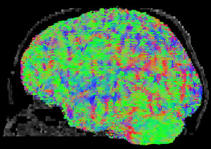
Tractography has become a valuable tool for neuroscientists because it is an in vivo way to examine white matter connectivity in the human brain, and is individualized to the particular anatomy of each subject. This avoids some of the difficulties of voxelwise approaches, and allows you, for example, to compare the properties of analogous white matter tracts across individuals even in the presence of large baseline differences in brain structure.
In a standard approach (below), the initial set of all the streamline “fibers” in the brain is pruned down through the use of multiple inclusion masks (orange) to result in a virtual dissection of the white matter tract of interest (here, the left corticospinal tract). Color encodes directionality, with the maxim “XYZ = RGB” explaining that fibers running left-right will be colored red, anterior-posterior will be green, and inferior-superior will be blue.


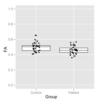
Once these virtual dissections have been performed on all of the subjects, the standard protocol is to then compare some measure of their quality between groups. For instance, we might investigate whether the mean FA – a metric related to myelination – is lower in a group of patients as compared to typical controls. A presentation of these results would look something like this:

While the above “tract-averaged” approach has led to many interesting results in the literature, it doesn’t capture the rich variation in FA that exists along white matter tracts. This variation is easy to see if we overlay FA onto the tract group (instead of directionality):

Using this corticospinal tract dissection as an example, the within-tract variability in FA might be something like ±0.14 (SD). This far exceeds both the between-subject variability in tract-averaged FA (something like ±0.03), as well as the tract-averaged effect sizes that are reported in the literature (effects of 0.03-0.05 are typical). Further, we can see that the greatest component of the within-tract variance exists along the longitudinal axis of the curving tract spine. This suggests that developing ways to analyze DTI metrics along tracts will allow us to:
- Improve detail in brain mapping studies
- Increase power to detect statistical effects (both in general, since the model residuals will be decreased in tracts showing this type of along-tract detail, but, in particular, the type of focal effects that could average themselves out and end up being missed in a tract-averaged analysis).
By performing an along-tract analysis, we can directly plot the along-tract variability that we visualized above. Individual streamlines are shown semi-transparently in the background. Overlaid on top is the along-tract cross-sectional mean FA±SD in blue. This should be compared to the red point-spread estimate in the middle, which represents the output of the tract-averaged approach. Not only does this uncover rich along-tract detail, but, as expected, the residual variance in the along-tract model is tighter at many locations along the tract since we are now accounting for real structure in our data that was ignored in the tract-averaged estimate.
For more info on performing this type of analysis, see: Single subject along-tract atlas

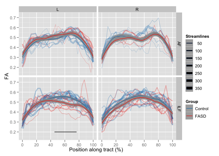
We can extend this idea to perform between-group analyses as well. Here we’re looking at a different tract (inferior longitudinal fasciculus), so the shape of the FA-position curve is different. We start by plotting the along-tract cross-sectional mean FA for each subject semi-transparently in the background (colored according to Group; # of streamlines encoded by varying line width). On top, we overlay the group means ±95% CI bands. Results of statistical hypothesis testing can also be annotated (here a black bar towards the bottom signifies areas of significant group differences.
Comparing this figure to the pair of boxplots that would result from a tract-averaged analysis (see above) makes it easy to see the potential advantages of performing an along-tract analysis. This example is a particularly useful demonstration, as the group effect is not an overall shift (like what would be tested for in the tract-averaged approach), but rather is isolated to a more focal region along the tract.
For more info on performing this type of analysis, see: Between-group along-tract analysis

Back to Wiki Home