Basic workflow

[See associated video]

This will take you through the standard way that the along-tract-stats tools are linked together. This page is an online version of the TrackVis/MATLAB Integration Demo that is included in the html directory when you download along-tract-stats.

Import tracts

Point MATLAB to the directory where the example data are stored. Replace the path here according to your own setup.

exDir = '/path/to/along-tract-stats/example';

Set paths to the .trk tract group file and the .nii.gz scalar MRI volume (e.g. FA map).

subDir  = fullfile(exDir, 'subject1');
trkPath = fullfile(subDir, 'CST_L.trk');
volPath = fullfile(subDir, 'dti_fa.nii.gz');

Read in the scalar FA map with FSL tools. (See $FSLDIR/etc/matlab)

volume = read_avw(volPath);

Read in the .trk file. You will get a header structure with fields from the .trk header, and a tracks structure array with an element for each streamline in the tract group.

[header tracks] = trk_read(trkPath)

Output:

header = 

                    id_string: 'TRACK '
                          dim: [192 192 55]
                   voxel_size: [1.2500 1.2500 2.5000]
                       origin: [0 0 0]
                    n_scalars: 0
                  scalar_name: [10x20 char]
                 n_properties: 0
                property_name: [10x20 char]
                     reserved: [508x1 char]
                  voxel_order: 'LPS '
                         pad2: 'LAS '
    image_orientation_patient: [1 0 0 0 -1 0]
                         pad1: '  '
                     invert_x: 0
                     invert_y: 1
                     invert_z: 0
                      swap_xy: 0
                      swap_yz: 0
                      swap_zx: 0
                      n_count: 734
                      version: 2
                     hdr_size: 1000


tracks = 

1x734 struct array with fields:
    nPoints
    matrix

Each structure in the tracks array contains fields for the number of points in that particular streamline, and the raw matrix of those points in mm coordinates [nPoints x 3]. If there were any whole-tract properties associated with the tract group, those would be listed here too.

tracks(1)
tracks(1).matrix

Output:

ans = 

    nPoints: 73
     matrix: [73x3 double]


ans =

  120.6250  105.6250    1.2500
  120.7721  105.9612    2.6684
  120.9682  106.2587    4.0910
  121.3031  106.5639    5.8192
  121.6318  106.9971    7.5074
  121.8181  107.5721    8.8092
  121.9920  108.3112   10.0386
  122.5117  109.9120   12.1337
  123.0796  111.1412   13.5634
  123.6738  112.3017   15.0360
  124.0613  113.0783   16.2544
  124.4113  113.7492   17.5483
  125.1193  114.7262   20.0167
  126.0355  115.4616   22.5005
  126.4101  115.7442   23.7574
  126.7523  116.0492   25.0180
  ...

Whole-tract statistics

Even though these tools are designed for looking at along-tract statistics, functions are stil included for determining the mean values of scalars, like FA, averaged across the whole tract. When setting up your workflow, it is useful to check these values to make sure they agree with what is reported in the tracking program (e.g. TrackVis). If they aren’t close, there is likely some orientation or related issue that needs to be worked out.

Determine traditional statistics collapsed across the whole tract.

[meanInt stdInt nVox] = trk_stats(header, tracks, volume, 'nearest')

Output:

Warning: Tracks don't have same length; padded with NaNs. 

meanInt =

    0.5863


stdInt =

    0.1370


nVox =

        1777

You can also look at streamline length.

lengths = trk_length(tracks);
mean(lengths)
std(lengths)

Output:

ans =

  121.7951


ans =

   13.1734

Interpolate streamlines

In order to look at FA along the tract, we first resample the streamlines so that they all have the same number of vertices spread evenly along their lengths. (However, see tie-at-center for a slightly more complex option that is usually preferable.) Here we use cubic B-spline interpolation and prescribe that we want 100 vertices in each streamline:

tracks_interp = trk_interp(tracks, 100);

Since the output of trk_interp is in matrix form (type help trk_interp to see this), we reformat the tracks back into a structure form.

tracks_interp_str = trk_restruc(tracks_interp);

Now we plot the tract group. The last input argument indicates the slice planes for volume overlays. Red markers indicate starting points. Note the random ordering of tracks, with some “starting” in the cortex and some in the brainstem.

figure, trk_plot(header, tracks_interp_str, volume, [95 78 4])
view([30 30])

Reorient streamlines

Since the default ordering of vertices within streamlines is arbitrary, we must flip some of the streamlines so that they all “start” at the same end of the tract. For some tracts, it is sufficient to specify a coordinate near the desired origin. For others (e.g. arcuate fasciculus, forceps major/minor, etc.), it is better to pick the origin manually for each subject. Since the corticospinal tract is pretty long, here we’ll specify a point near the brainstem. If we don’t provide a coordinate, the origin will be determined interactively [See video].

tracks_interp     = trk_flip(header, tracks_interp, [97 110 4]);
tracks_interp_str = trk_restruc(tracks_interp);

Plot the streamlines again to see that they have all been reordered.

figure, trk_plot(header, tracks_interp_str, volume, [95 78 4])
view([30 30])

Extract scalars and collapse cross-sectionally

For each point along the streamlines in tracks_interp_str, we extract the corresponding voxel intensity from volume.

[header_sc tracks_sc] = trk_add_sc(header, tracks_interp_str, volume, 'FA');

Obtain the mean FA at the different “cross-sections” along the curving tract spine.

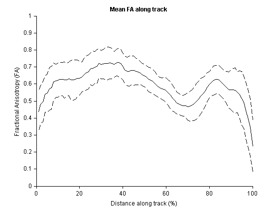
[scalar_mean scalar_sd] = trk_mean_sc(header_sc, tracks_sc);

Plot results

Finally, make a basic MATLAB plot of the mean FA value ± SD along the tract.

figure, hold on
plot(scalar_mean, 'k')
plot(scalar_mean+scalar_sd, 'k--')
plot(scalar_mean-scalar_sd, 'k--')

% Make the plot prettier
hold off, box off
xlim([0 100]), ylim([0 1])
title('\bf{Mean FA along track}')
xlabel('Distance along track (%)')
ylabel('Fractional Anisotropy (FA)')

Export tracts

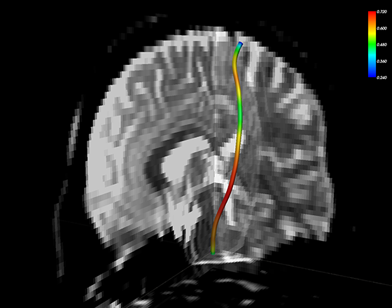
The mean streamline geometry (i.e. one streamline that represents the mean of all the original streamlines) can also be calculated.

track_mean = mean(tracks_interp, 3);

This average geometry can now be packaged up with the mean scalar values.

• Multiple scalars are allowed by the .trk format, which is very nice because it means we can also tag the vertices with other data like statistical significance values.
• A dummy streamline should be added with the desired display ranges for the scalars, if these exceed the ranges in the data (e.g. if you want the color bar for FA to be [0,1] even though the real data doesn’t fill that range).

track_mean_sc     = [track_mean scalar_mean];
%                         x y z   sc1
track_mean_sc(1:2,:,2) = [0 0 0   0;  %min
                          0 0 0.1 1]; %max
track_mean_sc_str = trk_restruc(track_mean_sc);

The header must be updated because now we only have 1 streamline (plus the 1 dummy range streamline) instead of many.

header_mean_sc         = header_sc;
header_mean_sc.n_count = 2;

Lastly, our results can be exported back out to a .trk file for visualization in TrackVis (this output is included in the example folder).

savePath = fullfile(exDir, 'CST_L_mean.trk');
trk_write(header_mean_sc, track_mean_sc_str, savePath)

Here we display the mean corticospinal tract geometry from the example subject, overlaid with the along-tract variation in FA [See video].