Alternative correspondence schemes

The main workflow in along-tract-stats uses B-spline resampling to ensure that every streamline has the same number of vertices spread in a regular fashion along its length. This is advantageous because it is then trivial to decide which vertices correspond (i.e. will be grouped together for statistical analysis) – all the first vertices in all the streamlines will be grouped together, all the second vertices in all the streamlines will be grouped together, etc.. However, there is nothing sacred about this choice, and there are certainly other nice methods that could be investigated. We have implemented 2 of these in trk_add_labs. These approaches are described fully in their original manuscripts (see links below), and also summarized more briefly in Colby et al. 2012. Here, instead, we will focus on some practical examples of how they can be used in along-tract-stats.

Preprocessing

Start by loading and processing the example data. This should look pretty familiar by now from the other tutorials.

exDir   = '/path/to/along-tract-stats/example';
subDir  = fullfile(exDir, 'subject1');
trkPath = fullfile(subDir, 'CST_L.trk');
volPath = fullfile(subDir, 'dti_fa.nii.gz');

[header tracks] = trk_read(trkPath);
volume          = read_avw(volPath);

Both of these methods require a “prototype” fiber. Here we will simply calculate the mean tract geometry derived from our B-spline resampling method, but other types of prototypes could be used as well.

nPts                = round(mean(trk_length(tracks)) / 4);
tracks              = trk_flip(header, tracks, [95 78 4]);
tracks_interp       = trk_interp(tracks, nPts, [], 1);
tracks_interp_str   = trk_restruc(tracks_interp);
[header tracks]     = trk_add_sc(header, tracks, volume, 'FA');
track_mean          = mean(tracks_interp, 3);
track_mean_str      = trk_restruc(track_mean);
header_mean         = header;
header_mean.n_count = 1;

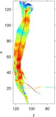
Now we can display the prototype fiber with the original tract group to see what we’ve got to work with. (Notice this way of shifting the prototype so it’s not completely obscured by all the other fibers)

trk_plot(header, tracks, [], [], 'scalar', 1)
trk_plot(header_mean, trk_restruc(bsxfun(@plus, track_mean, [20 0 0])), [], [], [], [], 1)
view([90 0])

“Distance map” method

Maddah et al. 2008

First let’s try this method from scratch. It will be relatively slow.

tic
[header tracks info] = trk_add_labs(header, tracks, track_mean_str, [], 'DM');
toc

Elapsed time is 7.890377 seconds.

Now we can try it again, while reusing the distance map, to see the nice speed boost.

opts = struct('info', info);

tic
trk_add_labs(header, tracks, track_mean_str, [], 'DM', opts);
toc

Elapsed time is 0.209356 seconds.

“Optimal point match” method

O’Donnell et al. 2009

For this method, let’s demonstrate how you can set some method-specific options.

opts = struct('tan_thresh', 0.4,...
              'euc_thresh', 0.3);
[header tracks] = trk_add_labs(header, tracks, track_mean_str, [], 'OP', opts);

Inspect results

Now we can inspect our results to see that these new labels have been added to our original tract group.

>> header.n_scalars

ans =

     3

>> header.scalar_name

ans =

FA                  
Label_DM            
Label_OP

>> tracks(1).matrix

ans =

  120.6250  105.6250    1.2500    0.4788    1.0000       NaN
  120.7721  105.9612    2.6684    0.5115    1.0000       NaN
  120.9682  106.2587    4.0910    0.3496    1.0000       NaN
  121.3031  106.5639    5.8192    0.6000    1.0000       NaN
  121.6318  106.9971    7.5074    0.5683    1.0000       NaN
  121.8181  107.5721    8.8092    0.5935    1.0000       NaN
  121.9920  108.3112   10.0386    0.6470    1.0000       NaN
  122.5117  109.9120   12.1337    0.7112    1.0000    1.0000
  123.0796  111.1412   13.5634    0.7249    1.0000    2.0000
  123.6738  112.3017   15.0360    0.6109    2.0000    2.0000
  124.0613  113.0783   16.2544    0.6427    2.0000    3.0000
  124.4113  113.7492   17.5483    0.5634    3.0000    3.0000
  125.1193  114.7262   20.0167    0.6417    3.0000    4.0000
  126.0355  115.4616   22.5005    0.5662    4.0000    4.0000
  126.4101  115.7442   23.7574    0.5764    4.0000    4.0000
  126.7523  116.0492   25.0180    0.6750    5.0000    5.0000
  127.5067  116.8137   27.4111    0.5752    5.0000    5.0000
  127.9900  117.1731   28.7186    0.5957    6.0000    6.0000
  128.5231  117.4263   30.0296    0.7044    6.0000    6.0000
  129.0690  117.5639   31.2818    0.7492    6.0000    6.0000
  129.6115  117.6561   32.5407    0.8347    7.0000    7.0000
  130.6059  117.8519   35.0161    0.7857    7.0000    7.0000
  131.1773  117.9335   36.2949    0.7857    8.0000    8.0000
  131.8337  118.0222   37.5288    0.7763    8.0000    8.0000
  ...

Comparison plots

Finally, we can make correspondence plots for all three of these methods (See also Fig. 9 in Colby et al. 2012). The main take-home message is that they are all able to successfully extract a large amount of the along-tract detail, while at the same time they show some method-specific variations that might make one more desirable than the rest for a given application.

% Along-tract stats
figure
subplot(1,3,1)
trk_plot(header, tracks_interp_str, [], [], 'rainbow')
view([90 0])
xlims = xlim;
ylims = ylim;
zlims = zlim;

% Distance map
subplot(1,3,2)
trk_plot(header, tracks, [], [], 'scalar', 2)
view([90 0])
xlim(xlims)
ylim(ylims)
zlim(zlims)

% Optimal point match
subplot(1,3,3)
trk_plot(header, tracks, [], [], 'scalar', 3)
view([90 0])
xlim(xlims)
ylim(ylims)
zlim(zlims)