Home

Welcome to the GW-SignalGen wiki!

Blog: Time and Frequency Analysis Methods on GW Signals

Notes by X. Li

1. Revisit Continuous Fourier Transform and Discrete Fourier Transform

Continuous Fourier Transform:

​ $$ X(f)=\int_{-\infty}^{\infty}x(t) e^{-j2\pi ft}dt $$

Discrete Fourier Transform:

$$ X(k)=\sum_{n=1}^{N-1} x(n)e^{-j2\pi kn/N} $$

where we let $$ \frac{k}{N}\equiv f $$ and $$ n \equiv t $$

2. Chirp Z Transform

The chirp Z-transform (CZT) is a generalization of the discrete Fourier transform (DFT). While the DFT samples the Z plane at uniformly-spaced points along the unit circle, the chirp Z-transform samples along spiral arcs in the Z-plane, corresponding to straight lines in the S plane.[1][2] The DFT, real DFT, and zoom DFT can be calculated as special cases of the CZT. ( - Wikipedia)

To obtain DCZT from DFT, we introduce $$ W^{kn}=e^{-j2\pi kn/N} $$ where $$ W^{kn}=W^{k^{2}/2}+ W^{n^{2}/2} + W^{-(k-n)^{2}/2} $$ thus, the DFT becomes $$ X(k)=W^{k^{2}/2}\sum_{n=1}^{N-1} x(n)W^{n^{2}/2}W^{-(k-n)^{2}/2} $$ where a complex chirp is introduced via $$ W^{n^{2}/2} $$

Discrete Chirp Z Transform (*to be verified):

$$ X(k)=e^{-j\pi k^{2}/N}\sum_{n=1}^{N-1} x(n)e^{-j\pi n^{2}/N} e^{j\pi(k-n)^{2}/N} $$

Compute with FFT & IFFT:

$$ X(k)=W^{k^{2}/2}IFFT[FFT(x(n)W^{n^{2}/2})FFT(W^{-(k-n)^{2}/2})] $$

Some notes:

When computing using FFT, the signal in the block is treated as periodic**(to be verified), however, the input signal itself does not need to be.

3. Gabor Transform

The Gabor transform is a special case of the short-time Fourier transform. It is used to determine the sinusoidal frequency and phase content of local sections of a signal as it changes over time. The function to be transformed is first multiplied by a Gaussian function, which can be regarded as a window function, and the resulting function is then transformed with a Fourier transform to derive the time-frequency analysis. ( - Wikipedia)

Continuous Gabor Transform:

$$ G_x(\tau, \omega)=\int_{-\infty}^{\infty}x(t)e^{-\pi (t-\tau)^{2}} e^{-j\omega t}dt $$

where the window function is a Gaussian in the form of $$ e^{-\pi \alpha(t-\tau)^{2}} $$ the width of which can be controlled via a scaling parameter α.

Thus the scaled Gabor is $$ G_x(\tau, \omega)=\sqrt[4]{\alpha}\int_{-\infty}^{\infty}x(t)e^{-\pi (t-\tau)^{2}} e^{-j\omega t}dt $$

Inverse Gabor Transform:

$$ x(t)=\int_{-\infty}^{\infty}G_x(\tau, \omega)e^{j\omega t}e^{\pi(t-\tau)^{2}}d\omega/(2\pi) $$

Gabor Expansion:

$$ y(t)=\sum_{m=-\infty}^{\infty}\sum_{n=-\infty}^{\infty}C_{nm}g_{nm}(t) $$

Discrete Gabor Transform (*to be verified):

$$ y(k)=\sum_{m=1}^{M-1}\sum_{n=1}^{N-1}.... $$

4. S Transform

The S transform is a generalization of the short-time Fourier transform (STFT), extending the continuous wavelet transform and overcoming some of its disadvantages. Modulation sinusoids are fixed with respect to the time axis; this localizes the scalable Gaussian window dilations and translations in S transform. The S transform doesn't have a cross-term problem and yields a better signal clarity than Gabor transform. ( - Wikipedia)

Continuous S Transform:

$$ S_x(\tau, \omega)=\int_{-\infty}^{\infty}x(t)|\omega|e^{-\pi (t-\tau)^{2}\omega^{2}}e^{-j2\pi \omega \tau}dt $$

Inverse S Transform:

$$ x(t)=\int_{-\infty}^{\infty}[\int_{-\infty}^{\infty}S_x(\tau, \omega)d\tau]e^{j2\pi \omega t}d\omega $$

Spectral Form:

$$ S_x(\tau, \omega)=\int_{-\infty}^{\infty}X(\omega+\alpha)e^{-\pi \alpha^{2}/\omega^{2}}e^{j2\pi \alpha \tau}d\alpha $$

where X(t) represents the Fourier Transform. (Convolution is used to get this spectral form)

Let $$ \tau = n\triangle_T, \omega = p\triangle_F,\alpha=p\triangle_T $$ We obtain the

Discrete S Transform:

$$ S_x(n\triangle_T, p\triangle_F)=\sum_{p=0}^{N-1}X[(p+m)\triangle_F]e^{-\pi p^{2}/m^{2}}e^{j2\pi pm/N} $$

Implementation:

  Step1.Compute 
  
    
    {\displaystyle X[p\Delta _{F}]\,}
  
X[p\Delta _{{F}}]\, 

  loop{
     Step2.Compute
  
    
    {\displaystyle e^{-\pi {\frac {p^{2}}{m^{2}}}}}
  
e^{{-\pi {\frac  {p^{2}}{m^{2}}}}}for 
  
    
    {\displaystyle f=m\Delta _{F}}
  
f=m\Delta _{{F}}

     Step3.Move 
  
    
    {\displaystyle X[p\Delta _{F}]}
  
X[p\Delta _{{F}}]to
  
    
    {\displaystyle X[(p+m)\Delta _{F}]}
  
X[(p+m)\Delta _{{F}}]

     Step4.Multiply Step2 and Step3 
  
    
    {\displaystyle B[m,p]=X[(p+m)\Delta _{F}]\cdot e^{-\pi {\frac {p^{2}}{m^{2}}}}}
  
B[m,p]=X[(p+m)\Delta _{{F}}]\cdot e^{{-\pi {\frac  {p^{2}}{m^{2}}}}}

     Step5.IDFT(
  
    
    {\displaystyle B[m,p]}
  
B[m,p]).
  Repeat.}

5. Constant Q Transform

CQT transforms a data series to the frequency domain. It is related to the Fourier transform[1] and very closely related to the complex Morlet wavelet transform.[2]

The transform can be thought of as a series of filters f**k, logarithmically spaced in frequency, with the k-th filter having a spectral width δf**k equal to a multiple of the previous filter's width:

where δf**k is the bandwidth of the k-th filter, fmin is the central frequency of the lowest filter, and n is the number of filters per octave. ( - Wikipedia)

6. Implementation on Chirp Signal (Windowed FFT - Tukey window)

In [1]:

import numpy as np
import matplotlib.pyplot as plt

In [2]:

dt = 0.001
t = np.arange(0,3,dt)
f0 = 50
f1 = 250
t1 = 2
x = np.cos(2*np.pi*t*(f0 + (f1 - f0)*np.power(t, 2)/(3*t1**2)))

fs = 1/dt

#Chirp signal
plt.plot(t, x)

In [3]:

from scipy import signal

In [4]:

freqs, times, spectrogram = signal.spectrogram(x)

#Scipy PSD Power Spectral Density
freqs, psd = signal.welch(x)

plt.figure(figsize=(5, 4))
plt.semilogx(freqs, psd)
plt.title('PSD: power spectral density')
plt.xlabel('Frequency')
plt.ylabel('Power')
plt.tight_layout()

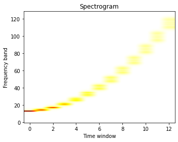
#Scipy Spectrogram
freqs, times, spectrogram = signal.spectrogram(x)

plt.figure(figsize=(5, 4))
plt.imshow(spectrogram, aspect='auto', cmap='hot_r', origin='lower')
plt.title('Spectrogram')
plt.ylabel('Frequency band')
plt.xlabel('Time window')
plt.tight_layout()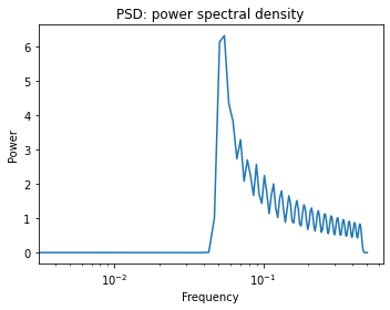

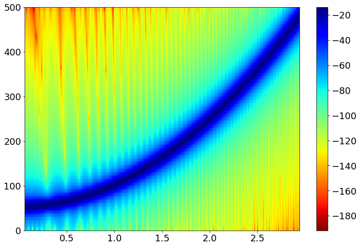
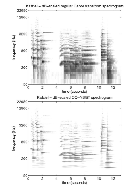
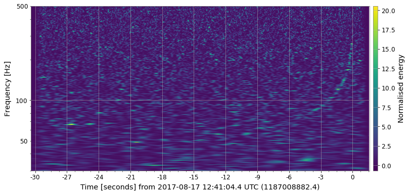
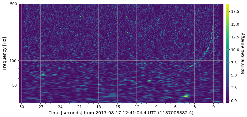
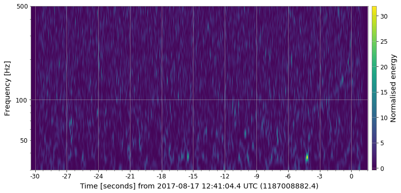
7. On the implementation of Time-Frequency Analysis for CNN

Constant Q Transform's high resolution at low frequencies is desirable in many cases for accurate analysis of the signal in both the time and frequency domain. However, when applying CQT for the purpose of identifying specific features on a spectrogram, high resolution in certain directions also means less obvious feature representation in certain cases (this assumption is highly dependent on the type of data you have). The Q range also affects the result significantly.

Some examples on GW chirp signal:

8. Resources on CQT

Invertible CQT: https://www.univie.ac.at/nonstatgab/cqt/index.php (Useful for the Spectrogram Denoising and Time-series parameter estimation)

Gabor Wavelets (bob package): https://pythonhosted.org/bob.ip.gabor/guide.html#gabor-wavelets

Window Functions (Wikipedia): https://en.wikipedia.org/wiki/Window_function

On the discrete Gabor transform and the discrete Zak transform: http://www.martinbastiaans.org/pdfs/sigpro.pdf