-
Notifications
You must be signed in to change notification settings - Fork 0
B. How to run the code
a. Provide the correct values to the DATA_DIR, SCRIPTS_DIR and ATLAS_DIR variables in utils/variables.py.
-
DATA_DIR: folder where you want to download the HCP dataset and perform all necessary analyses -
SCRIPTS_DIR: folder where you downloaded this repository -
ATLAS_DIR: folder where you placed the Schaefer atlas sub-folder.
b. provide your XNAT central user and password in utils/variables.py.
-
XNAT_USER: provide your username -
XANT_PASSWORD: provide your password
c. Similarly, you also need to provide the correct values for equivalent bash variables in Notebooks/common_variables.sh
-
DATA_DIR: folder where you want to download the HCP dataset and perform all necessary analyses -
SCRIPTS_DIR: folder where you downloaded this repository -
ATLAS_DIR: folder where you placed the Schaefer atlas sub-folder.
To run this code you will need two separate conda environments:
a. pyxant_env: This environment is used by notebook N00_DownloadDataFromHCPXNAT. This notebook downloads all the necessary data from XNAT Central using the pyxnat library. Because this library is not compatible with the latest version of other libraries used in this work, we need to create a separate environment just for this first notebook. A .yml file with the description of this first environment is provided in env_files/pyxnat_env.yml
b. hcp7t_fv_sleep_env: This environment is valid for all other notebooks. A .yml file with the description of this second environment is provided in env_files/hcp7t_fv_sleep_env.yml
Notebook N00_DownloadDataFromHCPXNAT contains the necessary code to downlaod most necessary data files from XNAT Central.
This notebook used the pyxant_env environment.
Many cells on this notebook will take a long time (over one hour). Be ready for that with a nice cup of coffee.
In addition, for the purpose of running HAPPY and looking at across-slice amplitude profile, we also need to download the raw, un-preprocessed data. This is done via Notebook N03b_DownloadOrig.
Notebook N01_QA will help us identify resting-state runs with issues such as missing ET data, ET files that do not load correctly, or have an incorrect number of volumes. Those will not be used in further analyses. This notebook will write a dataframe with this information that it is used in subsequent notebooks to load only valid data.
Notebook N02_ET-Preprocessing does all the pre-processing of the ET data as described in the manuscript. During the pre-processing, we detected a couple extra issues with a few runs. Namely, three runs did not have complete ET timeseries and 4 runs did not have information to permit synchronization of ET and fMRI data. At the completion of this notebook, you should have fully pre-processed ET traces stored in Resources/ET_PupilSize_Proc_1Hz_corrected.pkl for the 561 runs that passed all QA controls.
Notebook N03a_LabelScans_DrowsyAwake will label runs with eyes closed less than 95% of the time as "awake", and runs with eyes closed between 20% and 90% as "drwosy". The rest of the runs will be discarded. Those labels will be used in many subsequent analyses. This notebook also generates main figures 1 and 3.
| Figure 1 | Figure 3 |
|---|---|
 |
 |
This operation is also conducted by notebook N03a_LabelScans_DrowsyAwake. This notebook generates two pickle files Resources/EC_Segments_Info.pkl and Resources/EO_Segments_Info.pkl that contain information about every single EC and EO segment. Such information includes, among others, a unique identifier per segment (used to name files), segment onset, segment offset and segment duration.
To ensure the fluctuations observed here are of the same etiology as those reported by Fultz et al., we decided to look at across-slice intensity profiles using a subset of un-preprocessed scans. Those scans are characterized by low motion and long periods of eye closure. Notebook N03c_Inflow_Profile_Analysis and associated N03c files perform these set of analysis. They also contain the code to generate Figure 2.
| Figure 2 |
|---|
 |
Next, notebook N03d_Extract_ROI_TS.CreateSwarm will create the following outputs:
-
DATA_DIR/ALLfolder where to output files -
ALL_T1w_restore_brain.nii.gz: average of all T1s -
ALL_T2w_restore_brain.nii.gz: average of all T2s -
ALL_EPI_firstvols.nii.gz: average of the first volume of all rest scans in MNI space -
ALL_ROI.V4.mPP.nii.gz: group-level FV mask. -
ALL_ROI.V4lt.mPP.nii.gz: group-level lower half of FV mask.
In addition, this notebook will also create all necessary batch jobs to extract representative timeseries for the different versions of the FV mask, but also for the global signal and eroded WM. It will do this using the minimally preprocessed data.
NOTE: This part of the analyses rely on AFNI and scripts are designed to be run in a parallel computer cluster. They may need to be modified for your own computing environment.
Comparison of representative timeseries obtain on original data using manually drawn ROIs vs. minimally pre-processed data using the group average FV mask were conducted using notebook N03e_PartialVolumeEffects.
NOTE: This part of the analyses rely on AFNI and scripts are designed to be run in a parallel computer cluster. They may need to be modified for your own computing environment.
Because physiological traces are not available for this portion of the HCP dataset, we relied on the software package "HAPPY" to extract them directly from the fMRI data. This is done via notebook N04a_Run_Happy and associated files. Notebook N04a_Run_Happy is also where we generate supplementary figure 2.
Once cardiac traces are available, spectral analyses of those and statistical comparisons reported in figure 4 were conducted with notebook N04b_CardiacSignal_Analyses
| Figure 4 | Supp. Fig. 2 |
|---|---|
 |
 |
Notebooks N05a_Preproc_ROIs_STEP01 and N05a_Preproc_ROIs_STEP02 will create a series of subject-specific masks that will be used in subsequent analyses. These include:
-
ROI.WM_e2.nii.gz: WM eroded mask -
ROI.Va_e.mPP.nii.gz: eroded ventricular system mask -
ROI.compcorr.mPP.nii.gz: mask used for CompCor method (e.g., extraction of physiological regressors) -
ROI.GM_e.mPP.nii.gz: eroded GM mask -
ROI.FB_e.mPP.nii.gz: eroded full brain mask
Finally, these notebooks are also in charge of creating the final version of the 7 Network Schaeffer atlas that only contains ROIs sufficiently covered by the FOV of all scans. This is mostly done in STEP02.
NOTE: This part of the analyses rely on AFNI and scripts are designed to be run in a parallel computer cluster. They may need to be modified for your own computing environment.
Notebook N06_mPP_postProcessing.CreateSwarm will run a few different pre-processing pipelines described in the manuscript (i.e., basic, compcor). In particular, the following outputs are generated
-
${RUN}_BASIC.nii.gz| BASIC Pipeline: Blur (4mm) + Scaling + Regression (Motion + 1st Der Motion + Polort) + Bandpass [0.01 - 0.1 Hz] -
${RUN}_BASICnobpf.nii.gz| BASIC (no filtering) Pipeline: Blur (4mm) + Scaling + Regression (Motion + 1st Der Motion + Polort). This is created so that we can run rapidtide on the BASIC pipeline. Filtering needs to be done in rapidtide so that it can do statistics appropriately. -
${RUN}_AFNI_COMPCOR.nii.gz| AFNI Compcorr (deprecated): Blur (4mm) + Scaling + Regression (motion + 1st der mot + legendre 5 + 3 PCAs lat vents) + Bandpass [0.01 - 0.1Hz] -
${RUN}_AFNI_COMPCORp.nii.gz| AFNI Compcorr+ (deprecated): Blur (4mm) + Scaling + Regression (motion + 1st der mot + legendre 5 + 3 PCAs lat vents + 4th Ventricle) + Bandpass [0.01 - 0.1Hz] -
${RUN}_Behzadi_COMPCOR.nii.gz| COMPCOR Pipeline: Blur (4mm) + Scaling + Regression (motion + 1st der mot + legendre 5 + 5 PCAs CSF & WM) + Bandpass [0.01 - 0.1Hz].
NOTE: This part of the analyses rely on AFNI and scripts are designed to be run in a parallel computer cluster. They may need to be modified for your own computing environment.
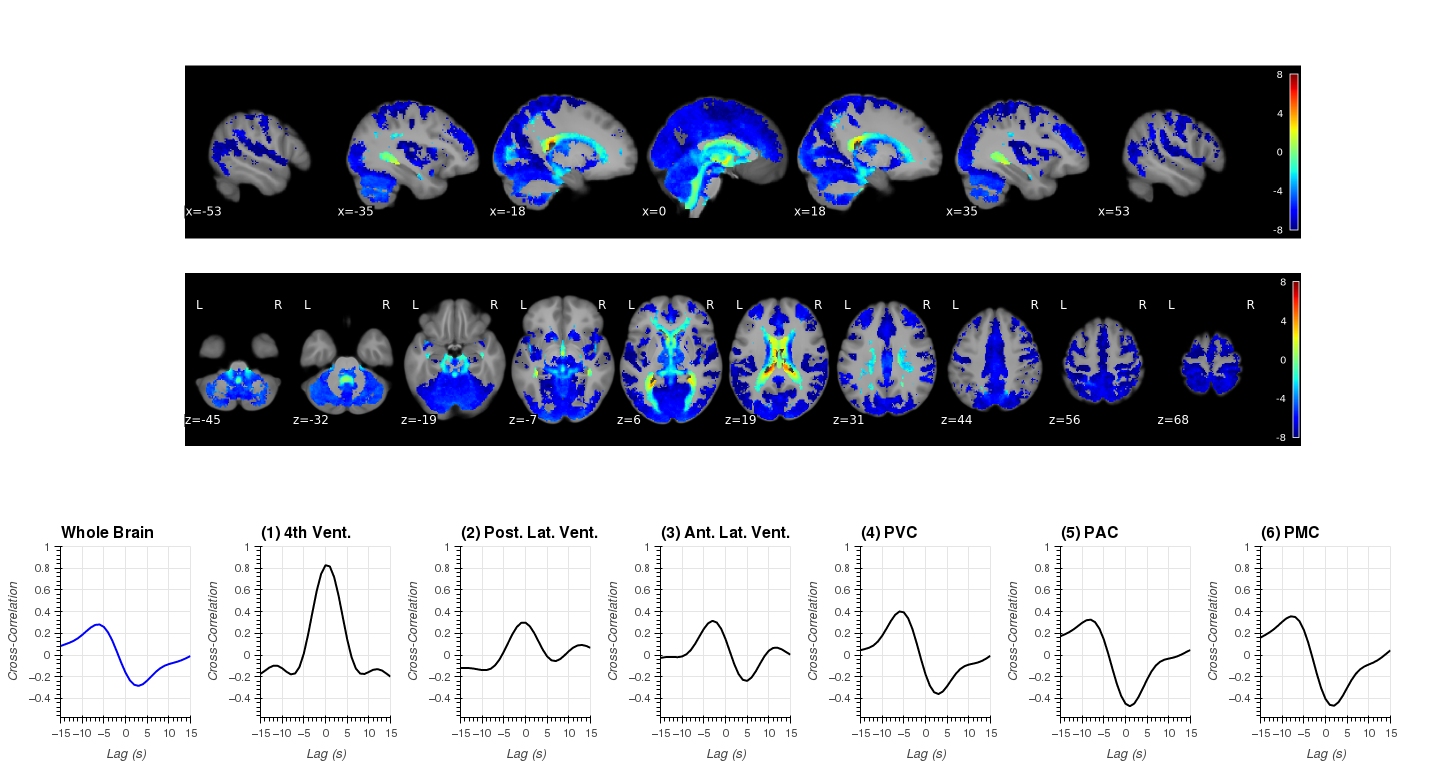
Notebooks N07_RapidTide.CreateSwarm will generate swarm files to run rapidtide on all 404 runs separately. In addition this notebook also contains the code to aggregate RapidTide results at the group level. Finally, it also contains the code to generate all the components that are part of Figure 8 (original submission).
Some important considerations here:
- RapidTide generates a lot of outputs. We will delete most of them (as we don't use them).
- We will only keep (and report) results for p<0.05.
- Group-level results only take into account voxels for which at least half the sample showed significance (RapidTide).
| Figure 8 |
|---|
 |
Notebooks N08_mPP_Peridiogram_FullRun will generate the swarm file to compute Power Spectral Density of all 404 scans using the Welch method. In addition, it will generate the group-level results where we compare for which frequencies we can observe a significant difference in PSD between Awake and Drowsy scans. This is reported as Panel A of Figure 5.
| Figure 5 - Panel A |
|---|
 |
Notebook N09_mPP_Peridiogram_Segments compute spectrograms for all continuous segments of eye closure and eye opening lasting at least 60 seconds. It also does the statistics to look for significant differences across segment types and generated Panel B for Figure 5.
| Figure 5 - Panel B |
|---|
 |
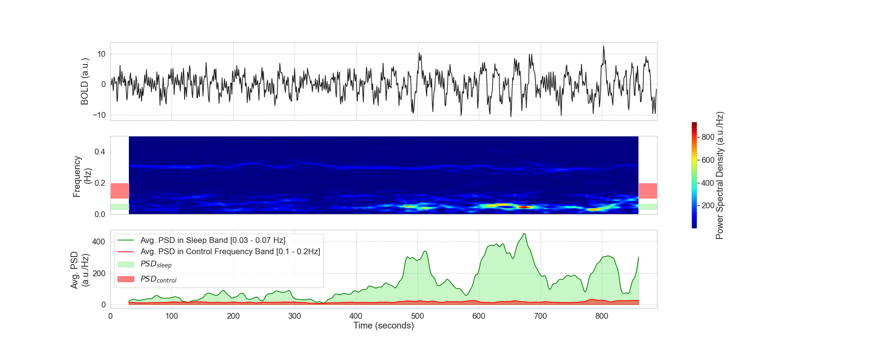
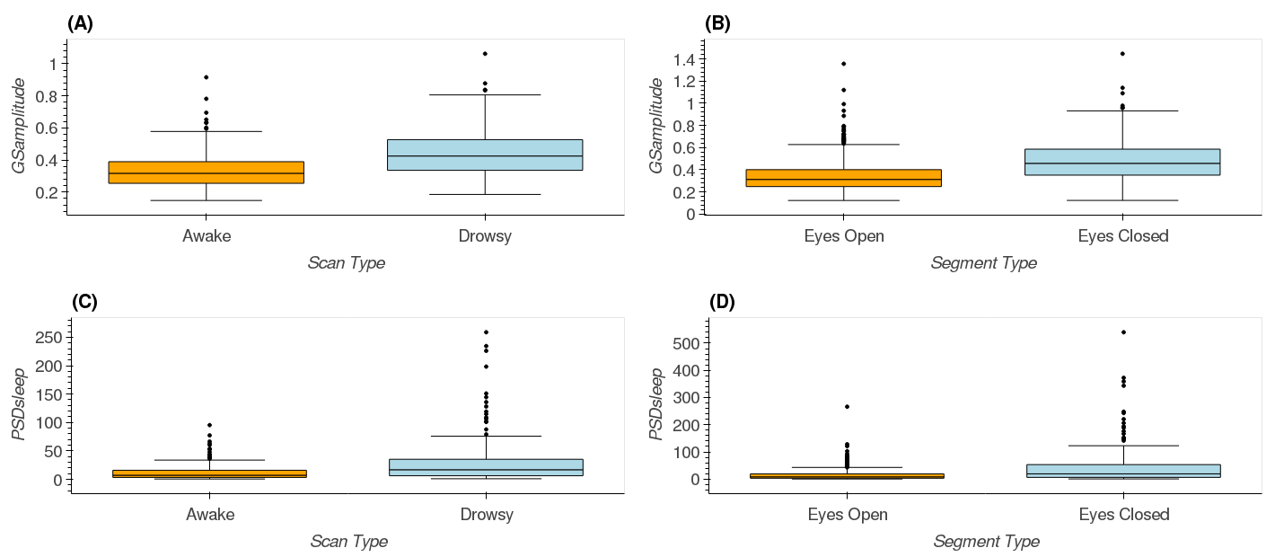
Notebooks N10_mPP_Spectrogram.CreateSwarm and N11_mPP_Scan_Spectrogram_Results were used to conduct spectrogram analyses on the FV signal. First, notebook N10_mPP_Spectrogram.CreateSwarm creates the swarm jobs that will compute the spectrogram and average PSD in sleep in control band for all 404 runs. Next, notebook N11_mPP_Scan_Spectrogram_Results will use these results to generate three manuscript figures:
- Figure 3 which is used as an example of how these analyses were conducted
- Figure 6 which shows how the PSD in the sleep band increases over scan time for drowsy scans but not for awake scans.
- Figure 9 which shows statistical differences in GSamplitude and PSDsleep between scan and segment types
- Figure 10 which shows the ranking of scans based on PSDsleep and Global Signal (GS)
| Figure 3 | Figure 6 |
|---|---|
 |
 |
| Figure 9 |
|---|
 |
| Figure 10 |
|---|
 |
Notebook N12_mPP_CorrMaps_Segments computes correlation between the FV signal and every other brain voxel. It does this separately for periods of eye opening and eye closure lasting more than 60 seconds. It also generates figure 07. This notebook contains information about AFNI commands that you will need to run on a console in order to get the different elements that form figure 07.
| Figure 7 |
|---|
 |
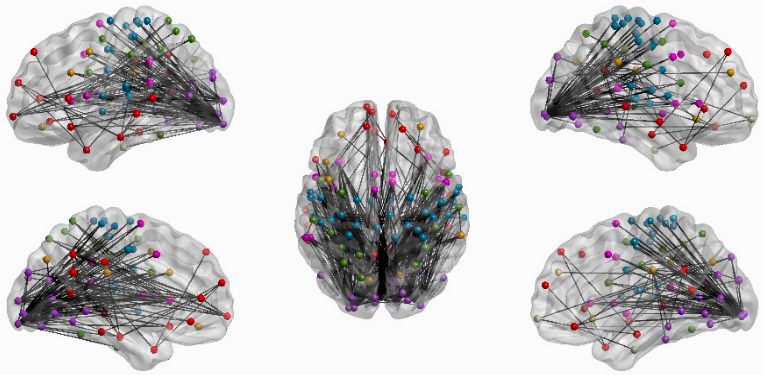
Notebook N13_FCMatrix_Schaefer200.CreateSwarm computes static FC matrices for Awake and Drowsy scans using different pre-processing pipelines. It presents these results in a dashboard. We take screen captures from this dashboard to generate panels in Figure 12. In addition, the notebook contains instructions on how to run Network-based Statistics (NBS) Analyses to detect changes in connectivity depending on how we try to account for the fluctuations of interest. Finally, it also provides instructions on how to load NBS results into BrainNetViewer to generate additional panels for Figure 12.
| Figure 12 - Dashboard Results |
|---|
 |
| Figure 12 - Brain Net Viewer Results |
|---|
 |
Notebook N14_LogisticRegression perform the logistic regression analyses reported on Figure 11, and produces the figure.
| Figure 11 |
|---|
 |