Home

JDemetra+ Nowcasting

Nowcasting is often defined as the prediction of the present, the very near future and the very recent past. The plug-in developed at the National Bank of Belgium helps to operationalize the process of nowcasting. It can be used to specify and estimate dynamic factor models and visualize how the real-time dataflow updates expectations, as for instance in Banbura and Modugno (2010). The software can also be used to perform pseudo out-of-sample forecasting evaluations that consider the calendar of data releases, contributing to the formalization of the nowcasting problem originally proposed by Giannone, et al. (2008) or Evans (2005).

Examples constructed or replicated with JDemetra+:

• Nowcasting Belgium, by de-Antonio-Liedo, NBB (R&D)
• US output-inflation interactions, by Charles, Maggi, Palate and de-Antonio-Liedo, NBB (R&D)

Building a simple nowcasting model

###1. Create a new model inside your workspace### Here we show how to generate a model. Go to the menu STATISTICAL METHODS and select the option Nowcasting. Select the type of nowcasting model desired. For example, "dynamic factor models".

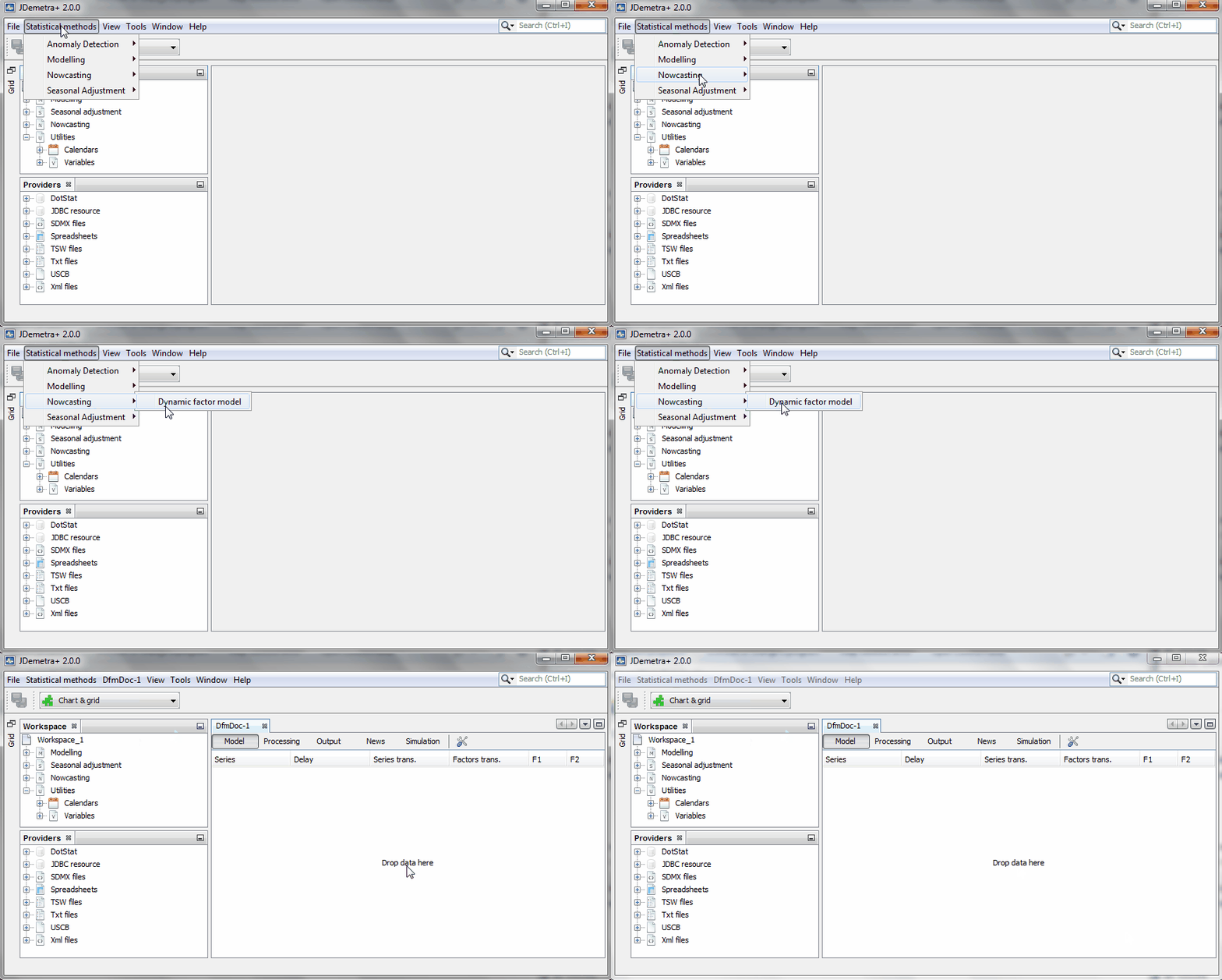
###2. Load the data###

Let's first load the data. Alternative formats are supported. If you work with data on excel, just make sure the dates are in the first column and the name of the series is in the first row:

• Go to the Providers window, select Spreadsheets (right click) and "Open" your file. The excel file with the data an be downloaded here: 
• Select the sheets that contains your data and copy each series or the whole sheet into the model space (use the drag and drop command).

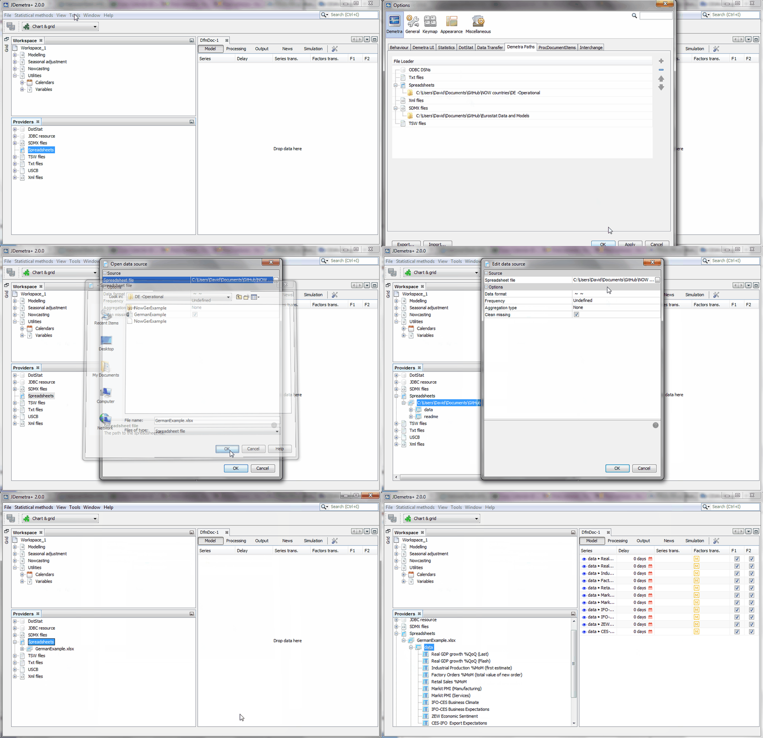
Tip: Make sure you remove the path specifying the location of the data to make sure JDemetra+ can access the data files also when they are stored in a different computer. You can simply specify the name of the file, as shown in this video, or a relative path, but you need to tell JDemetra+ in advance where to find the different types of data files. By selecting Tools>>Options>>Demetra paths, one can use as many paths as desired to organize the data.

###3. Model specification details###

The so-called state-space representation of the factor model is written as follows:

where the measurement equation links the N observables to the r underlying factors. Those factors, as shown in the second equation, follow a VAR of order p. This representation is valid in the case of missing observations or when monthly and quarterly variables are combined. In the latter case, it is simply assumed that the quarterly values are observed every three months.

####3.1. Define the measurement equation####

In this example we have variables observed at the monthly and quarterly frequencies. There is the option to transform the series in multiple ways, including first differences or seasonal adjustment. The likelihood of the model which is will be important for the estimation, will be given by the transformed data. However, the forecasts will be calculated for the raw data.

The link between the transformed time series and the factors can be very sophisticated. Three options are possible for the moment:

• Variables expressed in terms of monthly growth rates can be linked to a factor representing the underlying monthly growth rate of the economy if "M" is selected


• Monthly or quarterly variables that are correlated with the the underlying quarterly growth rate of the economy can be linked to a weighted average of the factors representing the underlying monthly growth rate of the economy. Such a weighted average is meant to represent quarterly growth rates, and it is implemented by selecting "Q":


• The variables can also be linked to the cumulative sum of the last 12 monthly factors. If the model is designed in such a way that the monthly factors represent monthly growth rates, the resulting cumulative sum boils down to the year-on-year growth rate. Thus, variables expressed in terms of year-on-year growth rates or surveys that are correlated with the year-on-year growth rates of the reference series should be linked to the factors using this link:


The factor loading structure can incorporate zero restrictions. Users should simply select which factors load on which variables. The following example helps to define a measurement equation for a very simple model for nowcasting German GDP:

####3.2. Define the transition equation#### The so-called transition equation is a representation of the r underlying factors in terms of a vector autoregressive model of order p. Both parameters can be determined by clicking on the tools option of Model tab.

The first unobserved factors in the sample is assumed either to be equal to zero or be consistent with a normal distribution with mean zero and a variance consistent with the unconditional variance of the VAR.

####3.3. Save your workspace and model specifications####

• The workspace can be saved by clicking on the FILE menu and selecting "save as". Let's first save the workspace with the name "NowGermany_24_11_2015", in reference to today's date.

• The name of our new model residing in our workspace ("Dfm1", by default) can be easily changed by applying the right click command. Select "Rename". Call it "Model r=2, p=3", in reference to the fact that the correlation among all variables is exclusively due to r=2 factors, which follow a VAR(p) of order p=3.

• As shown in the video, one may want to build a new model with identical properties as the previous one, but with one extra factor that loads on a variable that could be important for the German business cycle ([this claim can tested]). Go to the workspace window and right click on the model you want to modify. Select "Clone".

• You can see that a new model will be added to the list of models that already exist inside your workspace. Proceed as before (right click) with this new model, and select the option "Rename". Call it "Model r=3, p=3", in reference to the fact that it has now three factors following a VAR(3).

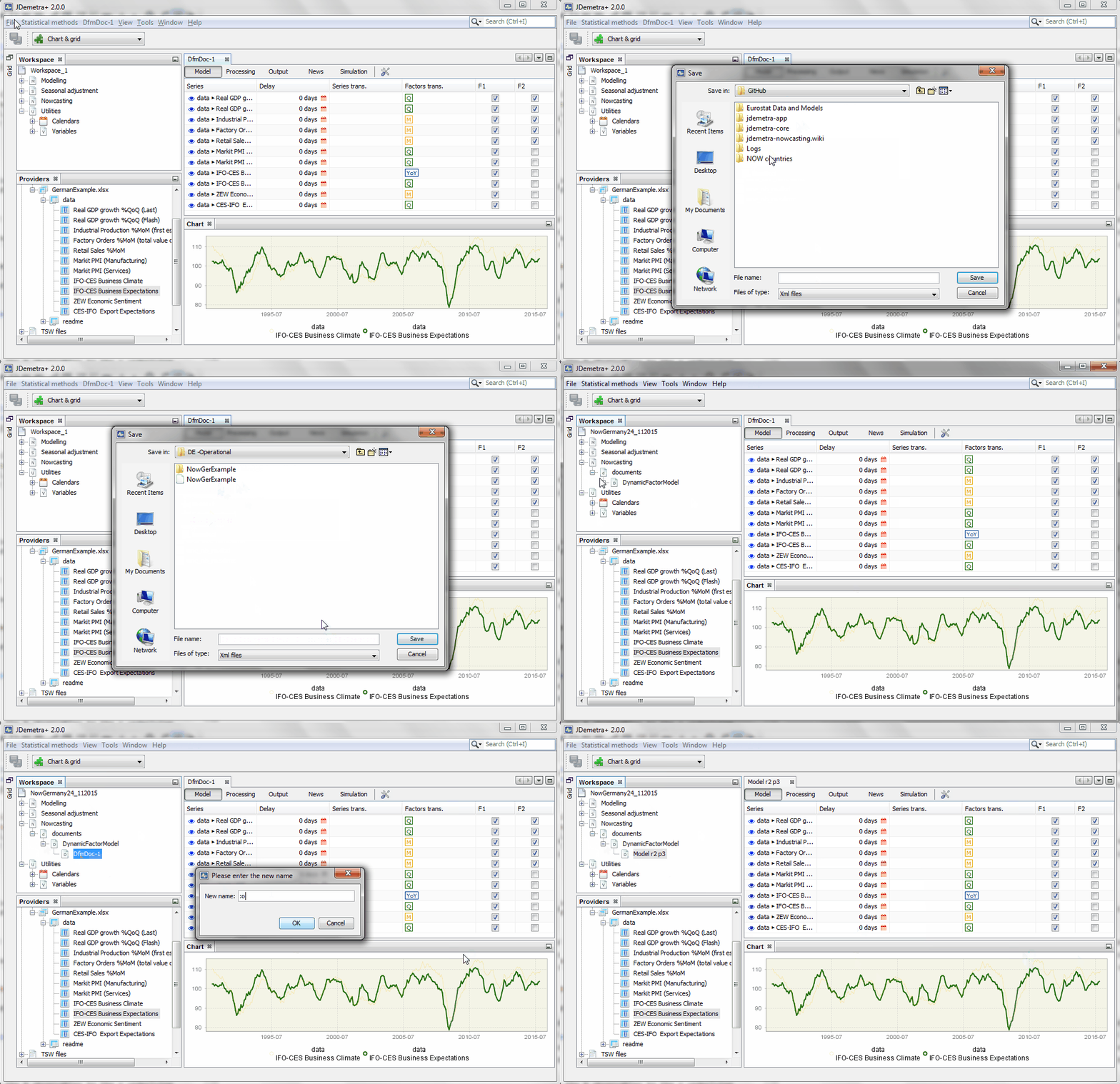
As a result of this step, an xml file with name "NowGermany_24_11_2015" is created. Such a file can be opened with JDemetra+. The file will access a folder with the same name that contain the two models we have specified, including the data.

###4. Opening an existing model###

A workspace can contain a large number of models. Let's consider a large dynamic factor model for the euro area proposed in the empirical application of one of the reference papers in the field of nowcasting with dynamic factor models. The largest model proposed by Banbura and Modugno (2010) accounts for the comovements of 101 indicators in terms of only five factors, r=5, following a VAR(p) with p=2.

Open the workspace BM2014_JAE, which contains three different versions of the same model. They only differ because of the sample used for the estimation of its parameters and the optimization method used to maximize the likelihood:

• The first one has been estimated with the first vintage of data used in the forecasting exercise proposed by the authors, which corresponds to October 1999. The estimation method is mainly based on a numerical optimization algorithm.
• The second model is exactly the same. The only difference is that it will be estimated using the Expectation-Maximization (EM) algorithm.
• The last model is again identical, but it is estimated using the whole sample.

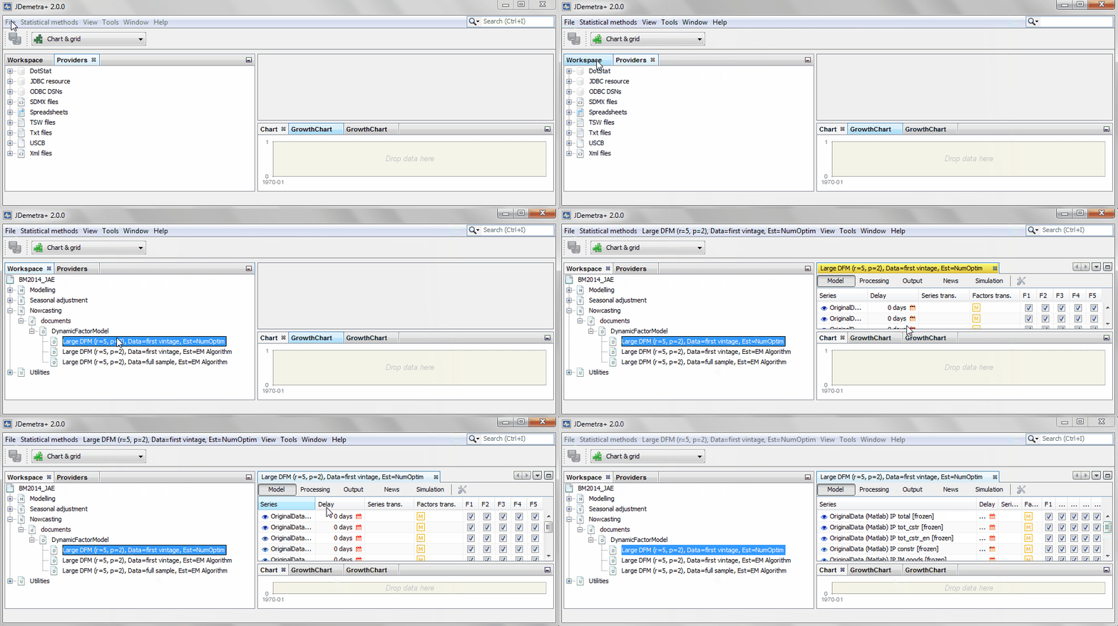
Users can specify and estimate as many different models as desired.

###5. Refreshing the data to be read by the model ### Here, we assume that the input data has already been refreshed in you Excel file. Now, such data has to be read by the model in order to update the forecasts. In this video, you can see that the data appears with the label "frozen", which disappears after the "refresh" action has been executed.

The option, "archive" can be used to freeze the data, but it locks the model at the same time. A model that is locked cannot be re-estimated and its specification cannot change. This is a way to make sure that someone borrowing the model does not change its properties accidentally. As it will be explained later on, re-estimating the model parameters is not necessary before updating the forecasts.

Tip: Archived models can be "unlocked" in order to re-estimate their parameters, but also to change their specification (N, r, and p). The "remove last archive" option redefines the model specification and data that had been saved before the last archive action.

Estimation

###1. Options ### By clicking on the tools option of Processing tab, you can combine select the options to estimate the parameters. Once selected, you can click on the estimation icon to proceed with the estimation. The estimation results can be deleted by clicking on the clear icon . This action ensures that previous results, including the sample means, are completely erased and are not used in the estimation as starting values.

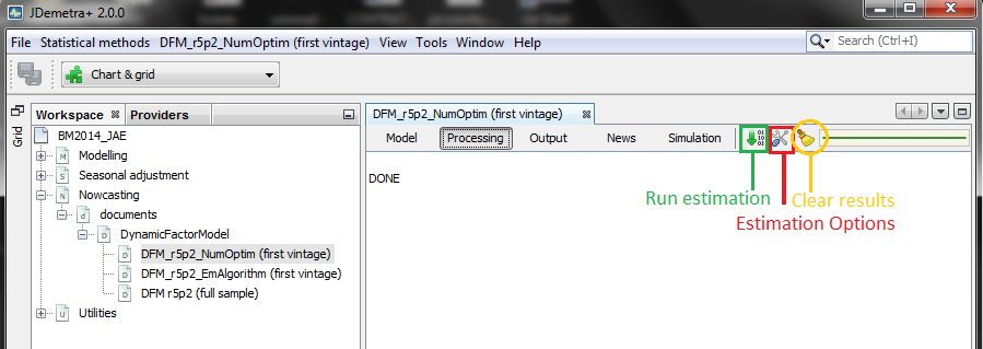
Numerical optimization and the EM algorithm play the most important role, and they can be combined. Let's look at two different ways to estimate the large dynamic factor model for the euro area described before, which has five factors (r=5) and two lags (p=2):

Numerical Optimization

• STEP 1: Principal components (PC) to extract the factors and run OLS regressions to get Z, R,A, and Q
• STEP 2:Use PC as starting value of a numerical optimization procedure (Levenberg-Marquardt) for the pseudo-likelihood (p=1). Not necessary to iterate until convergence: in this exaple, 15 iterations.
• STEP 3: Use the estimator obtained in the previous step as a starting value of the numerical optimization procedure for the true likelihood (p=2 in this example). The algorithm stops when the percentage likelihood does not increase by more than 1.0E-9. This value can be changed.


Expectations-Maximization algorithm

• STEP 1: Principal components (PC) to extract the factors and run OLS regressions to get Z, R,A, and Q
• STEP 2:Use PC as an initial condition for the EM algorithm and run it until the percentage likelihood does not increase by more than 1.0E-9. This algorithm, considers the analytical form of the first order conditions of the (expected) likelihood maximization problem, may converge very slowly when it is exploring the neighbourhood of the maximum likelihood solution.
• STEP 3: This final step may help to converge faster, but the results may be driven by the outcome of the previous EM step. We use the estimator obtained in STEP 2 as a starting value of the optimization procedure for the likelihood. Here, simplified model iterations is set to zero so that the likelihood continues improving until convergence.


Some Tips

• No rules of thumb. For very large models, it may be useful to use the EM algorithm before the numerical optimization procedure. However, for the relatively large model used here (101 variables available until 1999, r=5 and p=2), the numerical optimization strategy has proved to be more efficient, although this difference disappears when the full sample, which includes the Great Recession, is used in the estimation.


• Principal components. Both estimation options described here start with parameter values obtained with principal components. A final run of the EM algorithm is also possible, but useless in practice. Using the EM results as starting values for numerical optimization, as illustrated here, is standard practice, but not the other way round.

• Running the model without re-estimating the parameters. When all the options inside tools are checked out, the model parameters are not re-estimated, but only the Kalman filter and smoother are run to recalculate the factors without any modification in the model parameters. The estimation options become unchecked by default when you refresh your data. To put it simply, consider the factors as a weighted average of the data. When new data arrives, the factors can be recalculated using the same weights. This leads to new forecasts, even if the model parameters have not been re-estimated.

###2. Results ### [to be completed]