This repository includes the codes used in the 6 online lectures on SFC models delivered to the Central University of Finance and Economics and the Center for China Fiscal Development, Beijing, China, during November-December 2023 (see here and here). Specifically, it contains the R files that replicate PC, PC-EX1, BMW, and REG (toy) models from Godley and Lavoie, Monetary Economics. An Integrated Approach to Credit, Money, Income, Production and Wealth, including additional features. An empirically-calibrated version (named EMP), an input-output version (named IO-PC), and an ecosystem-augmented version (named ECO-PC) of Model PC are provided too.
Lectures' slides are available here:
-
Lecture A: Foundations of SFC Models for Economic Research (See also: Appendix_A)
-
Lecture B: A Toy Model with State Money and Bills
-
Lecture D: Multi-Country SFC Models
-
Lecture E: Ecological and Input-Output SFC Models
-
Lecture F: Empirical SFC Models (using
Bimets)
Lecture slides B, C, D, E and F are protected, and so is Appendix A. Contact me ([email protected]) to obtain the password. A more general description of lectures' contents is available below.
- 1 Introduction
- 2 Toy Models from Monetary Economics
- 3 Introducing input-output interdependencies
- 4 Introducing the ecosystem
- 5 Making it empirical
- 6 Useful links and resources
- 7 Lectures' flyer
In the last three decades, macroeconomic modelling has been dominated by Dynamic Stochastic General Equilibrium (DSGE) models. However, dissatisfaction with these models has been growing since the mid-2000s. Three primary weaknesses have been identified in DSGE models: unrealistic assumptions, a limited range of considerations, and poor data fit.
In response to these shortcomings, alternative models have emerged, aiming to address specific deficiencies. Computable General Equilibrium (CGE) models allow for broadening the scope but usually share key neoclassical assumptions with DSGE models. Leontief-like Input-Output (IO) models provide more room for a sound analysis of cross-industry interdependencies and the role of aggregate demand, but they still face limitations (as these models are static in nature, and their coverage of financial aspects is usually quite limited). Heterogeneous agent-based models, network analysis, and other complexity models offer novel perspectives. Lastly, Stock-Flow Consistent (SFC) models have gained traction, finding applications in empirical macroeconomic research by institutions like the Bank of England and the Italian Ministry of Economy and Finance.
The resurgence of interest in SFC models can be traced back to Wynne Godley's successful predictions of the U.S. crises in 2001 and 2007. Godley's work laid the foundation for modern SFC modelling. These models, rooted in national accounts and flow of funds, integrate financial and real aspects of the economy, allowing for the identification of unsustainable processes.
SFC models are akin to 'system dynamics' models, analysing complex systems over time, tracking flows, stocks, and utilising feedback loops. Basic SFC models have evolved into various forms, including Open-Economy or Multi-Area SFC models (MA-SFC), Ecological SFC models (ECO-SFC), Interacting Heterogeneous Agent-Based SFC models (AB-SFC), Input-output SFC Models (IO-SFC), and Empirical SFC Models (E-SFC).
Crucially, SFC models adhere to four accounting principles: flow consistency, stock consistency, stock-flow consistency, and quadruple book-keeping. The economy is represented by accounting matrices, identities reflecting the System of National Accounts, and dynamic equations defining the behaviour of each sector (usually based on rules of thumb and stock-flow norms).
Standard SFC models typically fall within the range of medium-scale macro-econometric dynamic models. These models are commonly formulated in discrete time using difference equations. However, continuous-time formulations using differential equations are also employed.
The simplicity or complexity of SFC models dictates the approach to solving them. The simplest models, featuring a limited number of equations, can be solved analytically by finding steady-state solutions. These solutions provide insights into the long-term behaviour of the model. More advanced SFC models, characterised by increased complexity and a larger number of equations, necessitate computational methods. Computer simulations become essential for understanding the dynamic interactions within the system. Numerical techniques, such as iterative methods, are employed to capture the intricate dynamics of these models.
Coefficients in SFC models play a crucial role in shaping model behaviour. Researchers have several options for determining these coefficients:
a) Fine-tuning: coefficients can be fine-tuned to achieve specific baseline scenarios, drawing insights from previous studies or selecting values from a reasonable range.
b) Calibration: researchers may calibrate coefficients to match the model's predictions with observed data, aligning the model with real-world economic conditions.
c) Estimation: econometric methods, including Ordinary Least Squares (OLS) and cointegration techniques, enable the estimation of coefficients from observed data, enhancing the model's empirical relevance.
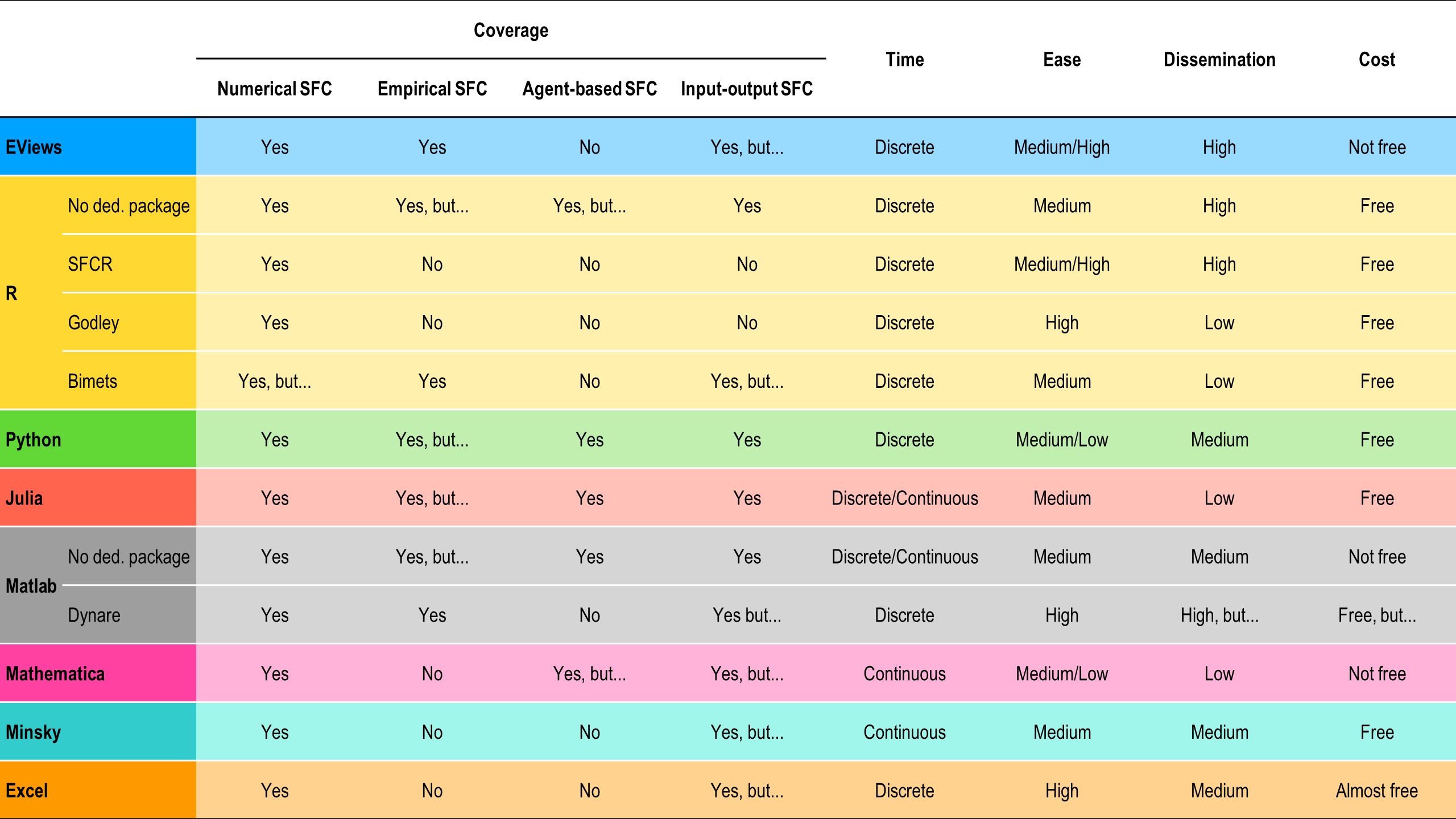
Unlike DSGE models, which often rely on a unified platform like Dynare, SFC modeling lacks a universally adopted program. The pioneering codes used in Godley and Lavoie's work were developed by Gennaro Zezza using EViews and Excel. However, the landscape has evolved over time. R (RStudio) has become the predominant programming environment for SFC modeling, owing to its flexibility and extensive capabilities. Dedicated R packages such as SFCR and Godley provide specialized tools for SFC modeling. Additionally, Bimets offers a platform for empirical SFC model development. Alternative programming languages, including MATLAB (with or without Dynare), Mathematica, Python, and Julia, find applications in SFC modeling, particularly for creating agent-based SFC models. Minsky, a software package developed by Steve Keen, stands out as a tool for visually modeling macroeconomic system dynamics.
Summing up, while there are many online resources today for those interested in engaging with SFC modeling, the community of SFC modelers lacks a portal that consolidates the produced material, which is abundant but still scattered (please refer also to the 6 Useful links and resources section).
This is one of the simplest SFC toy models. It is developed in chapter 4 of Godley and Lavoie (2007), "Monetary Economics. An Integrated Approach to Credit, Money, Income, Production and Wealth". PC stands for "portfolio choice", because households can hold their wealth in terms of cash and/or government bills.
Key assumptions are as follows:
-
Closed economy
-
Four agents: households, “firms”, government, central bank
-
Two financial assets: government bills and outside money (cash)
-
No investment (accumulation) and no inventories
-
Fixed prices and zero net profits
-
No banks, no inside money (bank deposits)
-
No ecosystem
We can also quickly review Model PC equations, as we will need them when for the upcoming Model REG, Model IO-PC, Model ECO-PC, and Model EMP:
Equation 1 - National income (identity):
Equation 2 - Disposable income (identity):
Equation 3 - Tax revenue (behavioural):
Equation 4 - Household wealth (identity):
Equation 5 - Consumption (hehavioural):
Equation 6 - Cash held by households (identity):
Equation 7 - Bills held by households (behavioural):
Equation 8 - Supply of bills (identity):
Equation 9 - Supply of cash (identity):
Equation 10 - Bills held by central bank (identity):
Equation 11 - Interest rate (behavioural):
Redundant equation:
The first step in developing the model in an R environment is to define the number of scenarios considered and the time span.
#Number of periods
nPeriods = 90

#Number of scenarios
nScenarios=3
The second step is to define and identity model coefficients. Parameters and exogenous variables are typically represented as scalars.
#Define coefficients
alpha2=0.4 #Propensity to consume out of wealth
lambda0 = 0.635 #Autonomous share of bills
lambda1 = 5 #Elasticity of bills demand to interest rate
lambda2 = 0.01 #Elasticity of bills demand to yd/v
theta=0.2 #Tax rate on income
In contrast, endogenous variables are modelled as matrices, where rows represent different scenarios and columns denote distinct periods.
#Define variables
b_cb=matrix(data=21.62,nrow=nScenarios,ncol=nPeriods) #Government bills held by central bank
b_h=matrix(data=64.87,nrow=nScenarios,ncol=nPeriods) #Government bills held by households
b_s=matrix(data=21.62+64.87,nrow=nScenarios,ncol=nPeriods) #Government bills supplied by government
cons=matrix(data=0,nrow=nScenarios,ncol=nPeriods) #Consumption
g=matrix(data=20,nrow=nScenarios,ncol=nPeriods) #Government expenditure
h_h=matrix(data=21.62,nrow=nScenarios,ncol=nPeriods) #Cash money held by households
h_s=matrix(data=21.62,nrow=nScenarios,ncol=nPeriods) #Cash money supplied by central bank
r=matrix(data=r_bar,nrow=nScenarios,ncol=nPeriods) #Interest rate on government bills
t=matrix(data=0,nrow=nScenarios,ncol=nPeriods) #Taxes
v=matrix(data=64.87+21.62,nrow=nScenarios,ncol=nPeriods) #Households wealth
y=matrix(data=0,nrow=nScenarios,ncol=nPeriods) #Income = GDP
yd=matrix(data=0,nrow=nScenarios,ncol=nPeriods) #Disposable income of households
Parameters and exogenous variables susceptible to shocks are also treated as matrices (or vectors), as they change over time.
#Define coefficients susceptible to shocks
alpha1=matrix(data=0.6,nrow=nScenarios,ncol=nPeriods) #Propensity to consume out of income (as matrix)
r_bar=matrix(data=0.025,nrow=nScenarios,ncol=nPeriods) #Interest rate (as matrix)
Once model coefficients and variables are defined, and before writing down the system of equations, three loops must be created to run the model:
-
The first loop defines the considered scenarios.
-
The second loop establishes the dynamic time span of the model.
-
The third loop iterates the model, ensuring the system of equations converges to its simultaneous solution.
The third loop is fundamental. Equilibrium solutions for the system of simultaneous equations are derived without relying on any dedicated package but rather through a sufficiently high number of iterations. In the absence of this loop, R would execute the code equation by equation, and the solution would depend on the specific order chosen.
#Choose scenario
for (j in 1:nScenarios){

  #Define time loop
  for (i in 2:nPeriods){

    #Define iterations
    for (iterations in 1:100){

      #Shock 1: higher interest rate
      if (i>=10 && j==2){r_bar[j,i]=0.035}

      #Shock 2: higher propensity to consume out of income
      if (i>=10 && j==3){alpha1[j,i]=0.7}

       #Determination of output - eq. 4.1
       y[j,i] = cons[j,i] + g[j,i]

       #Disposable income - eq. 4.2
       yd[j,i] = y[j,i] - t[j,i] + r[j,i-1]*b_h[j,i-1]

       #Tax payments - eq. 4.3
       t[j,i] = theta*(y[j,i] + r[j,i-1]*b_h[j,i-1])

       #Wealth accumulation - eq. 4.4
       v[j,i] = v[j,i-1] + (yd[j,i] - cons[j,i])

       #Consumption function - eq. 4.5
       cons[j,i] = alpha1[j,i]*yd[j,i] + alpha2*v[j,i-1]

       #Cash money - eq. 4.6
       h_h[j,i] = v[j,i] - b_h[j,i]

       #Demand for government bills - eq. 4.7
       b_h[j,i] = v[j,i]*(lambda0 + lambda1*r[j,i] - lambda2*(yd[j,i]/v[j,i]))

       #Supply of government bills - eq. 4.8
       b_s[j,i] = b_s[j,i-1] + (g[j,i] + r[j,i-1]*b_s[j,i-1]) - (t[j,i] + r[j,i-1]*b_cb[j,i-1])

       #Supply of cash - eq. 4.9
       h_s[j,i] = h_s[j,i-1] + b_cb[j,i] - b_cb[j,i-1]

       #Government bills held by the central bank - eq. 4.10
       b_cb[j,i] = b_s[j,i] - b_h[j,i]

       #Interest rate as policy instrument - eq. 4.11
       r[j,i] = r_bar[j,i]

      }
   }
}
In the R code block above, subscript
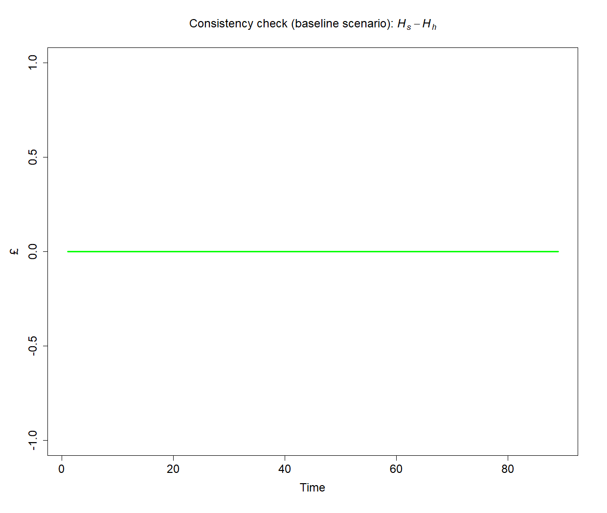
Lastly, any complete and coherent model must contain an equation that is redundant, meaning that it is logically implied by all the others (Walras' Law). While this equation must be excluded from the model (which is the reason it is sometimes called the hidden equation), it can be used to double-check its accounting coherence. More precisely, we use it to verify the consistency of the model in the baseline scenario, both numerically and graphically.
#Create consistency statement
aerror=0
error=0
for (i in 2:(nPeriods-1)){error = error + (h_s[1,i]-h_h[1,i])^2}
aerror = error/nPeriods
if ( aerror<0.01 ){cat(" *********************************** \n Good news! The model is watertight! \n", "Average error =", aerror, "< 0.01 \n", "Cumulative error =", error, "\n ***********************************")} else{
  if ( aerror<1 && aerror<1 ){cat(" *********************************** \n Minor issues with model consistency \n", "Average error =", aerror, "> 0.01 \n", "Cumulative error =", error, "\n ***********************************")}
  else{cat(" ******************************************* \n Warning: the model is not fully consistent! \n", "Average error =", aerror, "> 1 \n", "Cumulative error =", error, "\n *******************************************")} }

#Plot redundant equation
layout(matrix(c(1,2,3,4), 2, 2, byrow = TRUE))
par(mar = c(5.1+1, 4.1+1, 4.1+1, 2.1+1))
plot(h_s[1,2:nPeriods]-h_h[1,2:nPeriods], type="l", col="green",lwd=3,lty=1,font.main=1,cex.main=1.5,
     main=expression("Consistency check (baseline scenario): " * italic(H[phantom("")]["s"]) - italic(H[phantom("")]["h"])),
     cex.axis=1.5,cex.lab=1.5,ylab = '\u00A3',
xlab = 'Time',ylim = range(-1,1))Tip: If the symbol £ is not displayed correctly in your plots, use the Unicode character \u00A3 instead.
 ***********************************
 Good news! The model is watertight!
 Average error = 2.804979e-27 < 0.01
 Cumulative error = 2.524481e-25
 ***********************************
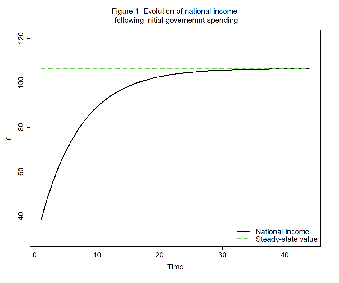
We can calculate the (quasi) steady state solution for national income
where
We can verify whether the model actually reaches the steady state as calculated above. The plot below confirms that it does:
The main code for replicating the baseline scenario can be found here.
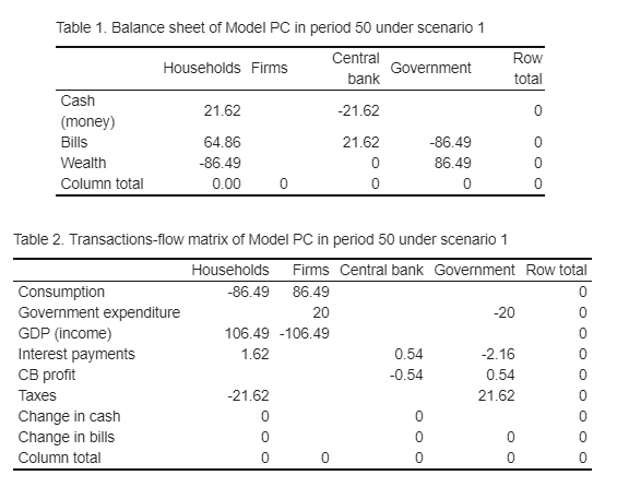
Crucial identities of the model are derived using the balance-sheet matrix and the transaction-flow matrix. These tables are also useful to double-check model consistency in each period. A few additional lines of code are enough to generate these tables automatically.
Tables are displayed in the Console (bottom-left pane in RStudio). For instance, we may want to verify what steady-state values are:
|             |      H|P  |CB     |G      | Tot|
|:------------|------:|:--|:------|:------|---:|
|Cash (money) |  21.62|   |-21.62 |       |   0|
|Bills        |  64.86|   |21.62  |-86.49 |   0|
|Wealth       | -86.49|   |0      |86.49  |   0|
|Column total |   0.00|0  |0      |0      |   0|

|                       |H      |P       |CB    |G     | Tot|
|:----------------------|:------|:-------|:-----|:-----|---:|
|Consumption            |-86.49 |86.49   |      |      |   0|
|Government expenditure |       |20      |      |-20   |   0|
|GDP (income)           |106.49 |-106.49 |      |      |   0|
|Interest payments      |1.62   |        |0.54  |-2.16 |   0|
|CB profit              |       |        |-0.54 |0.54  |   0|
|Taxes                  |-21.62 |        |      |21.62 |   0|
|Change in cash         |0      |        |0     |      |   0|
|Change in bills        |0      |        |0     |0     |   0|
|Column total           |0      |0       |0     |0     |   0|
Notice that these tables can be conveniently turned into HTML (and LaTeX) format (we refer again to the auxiliary code for the tables here).
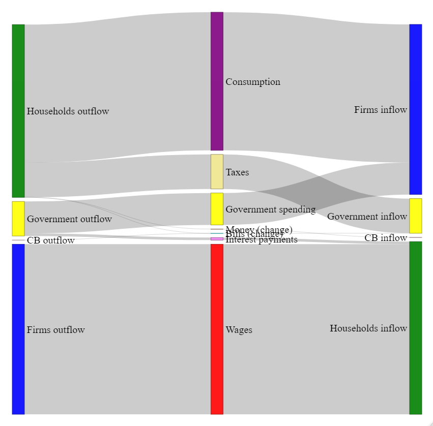
The code also allows for creating the Sankey diagram of transactions and changes in stocks (here).
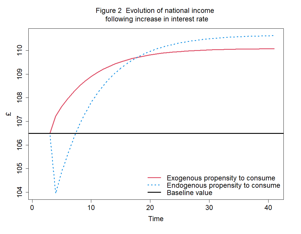
The baseline scenario is then compared with alternative scenarios, which are generated by shocks to exogenous variables and/or parameters. For instance, one may wonder what happens when the interest rate is increased:
As the figure above shows, the answer depends on the way we define the consumpion function (and other behavioural equations). While the red line refers to the standard model, the blue dotted line shows the evolution of national income when the propensity to consume out of income is a negative function of the interest rate:
with
When the propensity to consume is affected by the increase in the interest rate, national income reduces in the short run due to lower demand for consumer goods (paradox of thrift). However, in both scenarios, national income reaches a higher steady-state value in the long run. The reason is that lower consumption is associated with higher saving in each period, resulting in a higher stock of (target) wealth and bills held by households. This, in turn, implies higher interest payments from the government, leading to higher income.
The code for replicating the experiments can be found here. The expectations-augmented version of Model PC, named PCEX1, is available here. Differences between the two models can be identified by using this comparison file.
This is the simplest model explicitly including commercial banks. It is developed in chapter 7 of Godley and Lavoie (2007), "Monetary Economics. An Integrated Approach to Credit, Money, Income, Production and Wealth". BMW stands for "bank-money world", because there is only one kind of financial assets: bank deposits held by households. Firms’ investment in fixed capital is funded by bank loans and amortisation funds.
Key assumptions are as follows:
-
Closed economy and no ecosystem
-
Three agents: households, firms, banks
-
Assets and liabilities include: loans, deposits, tangible (or fixed) capital
-
Investment funded by loans and internal funds
-
Target capital to output ratio
-
Fixed prices and zero net profits
-
No State, no outside money (cash)
The main code for reproducing the experiments can be found here. A code that automatically generates SFC tables can be found here. The code for the Sankey diagram replicating the transactions-flow matrix is here. Lastly, the codes for a more advanced simulation of an SFC model, incorporating both state and bank money, are available here.
Open-economy or multi-area SFC models adopt a general equilibrium approach, accounting for the interaction of two economies engaged in the trade of goods. The entire system, representing the global economy, is closed, meticulously tracking all flows and stocks. Godley and Lavoie (2007) introduce and explore four distinct models:
-
Model REG: a toy model that examines two regions within the same country
-
Model OPEN: a toy model involving two separate countries
-
Model OPENFIX: an advanced model encompassing two countries under a fixed exchange rate regime
-
Model OPENFLEX: an advanced model dealing with two countries under a floating exchange rate regime
In this section, we will present and discuss Model REG, which is developed in chapter 6 of Godley and Lavoie (2007), "Monetary Economics. An Integrated Approach to Credit, Money, Income, Production and Wealth". REG stands for "regional", as the model considers two regions of the same country. Looking at its economic and financial structure, it is the very same of Model PC. The difference is that the economy is disaggregated into two regions, the North and the South.
Key assumptions are as follows:
-
Firms act as intermediaries for imported goods
-
Four agents: households, “firms”, government, central bank
-
Two financial assets: government bills and outside money (cash)
-
No investment (accumulation) and no inventories
-
Fixed prices and zero net profits
-
No banks, no inside money (bank deposits)
-
No ecosystem
The main code for reproducing the experiments can be found here. A code that automatically generates 2-region SFC tables can be found here. Lastly, the code for the Sankey diagram replicating the 2-region transactions-flow matrix is here. The codes for more advanced open-economy SFC models can be found here.
There are currently only a few prototype input-output SFC models, despite recent progress (Berg, Hartley, and Richters, 2015; Jackson and Jackson, 2021, 2023; Valdecantos, 2023). Integrating IO and SFC techniques poses challenges, but it is crucial for analysing both technical progress (Veronese Passarella, 2023) and the interaction of the ecosystem with the economy (Hardt and O’Neill, 2017).
Model IO-PC is an input-output extension of Model PC, where IO stands for "input-output structure."
In comparison to Model PC, additional assumptions include:
-
Two industries are considered (within the firms sector)
-
Only circulating capital is used
-
Technical coefficients are fixed
-
Each industry uses only one technique to produce one product
-
Prices are fixed
-
The composition of both consumption and government spending is exogenously defined
Based on these assumptions, a few additional equations are required to transform Model PC into Model IO-PC. Notice that scalars are represented using italic characters, whereas vectors and matrices are represented using non-italic characters hereafter.
Equation 12 - Column vector of exogenously-set unit prices (behavioural):
Equation 13 - Column vector defining composition of real consumption (behavioural):
Equation 14 - Column vector defining composition of real government expenditure (behavioural):
Equation 15 - Average consumer price (identity):
Equation 16 - Average price for the government (identity):
Equation 17 - Column vector of final demands in real terms (identity):
Equation 18 - Column vector of real gross outputs (identity):
Equation 1.A - Modified equation for national income (identity):
Equation 19 - Real consumption function (behavioural):
Equation 5.A - Nominal consumption (identity):
Equation 20 - Nominal government spending (identity):
Note: the superscript
While 12 to 20 are additional equations, equations 1.A and 5.A replace equations 1 and 5 of Model PC, respectively. The main code for developing Model IO-PC and running some experiments can be found here.
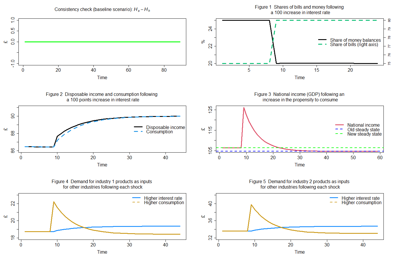
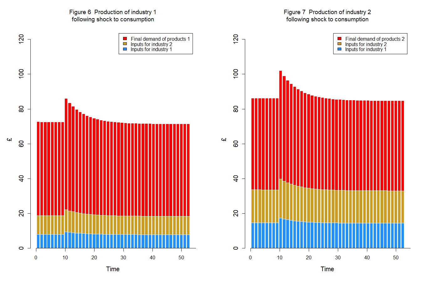
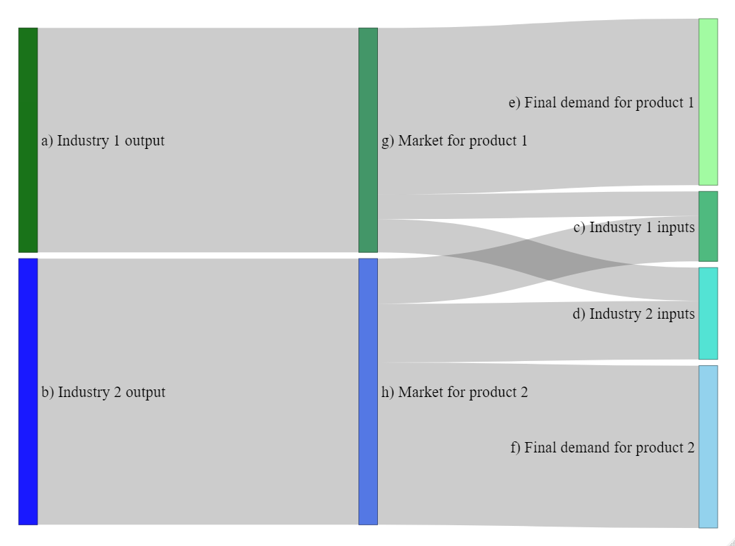
Variables displayed in figures 1 to 3 follow the same pattern as Model PC variables. However, Model IO-PC also allows tracking cross-industry demands for inputs (figures 4 and 5). A more detailed visualisation, highlighting the impact of final and intermediate demands on total outputs, is presented below in Figures 7 and 8:
A code that automatically generates SFC tables can be found here. This code allows for the generation of not only the BS and the TFM but also the input-output table of the economy.
The code for the Sankey diagram replicating the transactions-flow matrix is provided here. The same code also allows visualising cross-industry intedependencies, that is, the IO table of the economy.
Although the origins of ecological macroeconomics can be traced back to the inception of economics itself, early SFC models for economic research did not incorporate the ecosystem.
This gap was bridged in the late 2010s (Dafermos, Nikolaidi, and Galanis, 2016, 2018; Jackson and Victor, 2015). The primary characteristic of ecological SFC models is their integration of monetary variables (following Godley and Lavoie, 2008) with physical variables (in line with Georgescu-Roegen, 1971) in a consistent manner. Several ECO-SFC models have been developed since then.
Here we consider a simple extension of Model IO-PC, named Model ECO-PC, where ECO stands for "ecological". Additional assumptions are as follows:
-
there are 2 types of reserves: matter and energy
-
there are 2 types of energy: renewable and non-renewable
-
Resources are converted into reserves at a certain rate
-
Industrial CO2 emissions are associated with the use of non-renewable energy
-
Atmospheric temperature is a growing function of CO2 emissions
-
Both goods from industry 1 and industry 2 can be durable or non-durable
-
A share of durable goods (hence socio-economic stock) is discarded in every period
-
Both waste and emissions are produced only by the firm sector
Behavioural equations draw inspiration from the works of Dafermos, Nikolaidi, and Galanis (2016, 2018). The main model code is accessible here. The blocks providing the additional equations for the ecosystem are those included between line 228 and line 305. Firstly, extraction of matter and waste are modelled:
#Production of material goods
x_mat[j,i] = t(mu_mat[,]) %*% x[j,i,]

#Extraction of matter
mat[j,i] = x_mat[j,i] - rec[j,i]

#Recycled matter (of socioeconomic stock + industrial waste)
rec[j,i] = rho_dis*dis[j,i]

#Discarded socioeconomic stock
dis[j,i] = t(mu_mat[,]) %*% (zeta_dc[,] * dc[j,i-1,])

#Stock of durable consumption goods
dc[j,i,] = dc[j,i-1,] + beta_c[j,i,]*cons[j,i] - zeta_dc[,] * dc[j,i-1,]

#Socioeconomic stock
kh[j,i] = kh[j,i-1] + x_mat[j,i] - dis[j,i]

#Wasted socio-economic stock
wa[j,i] = mat[j,i] - (kh[j,i]-kh[j,i-1])
Secondly, energy use and CO2 emissions are considered.
#Energy required for production
en[j,i] = t(eps_en[,]) %*% x[j,i,]

#Renewable energy at the end of the period
ren[j,i] = t(eps_en[,]) %*% (eta_en[,]*x[j,i,])

#Non-renewable energy
nen[j,i] = en[j,i] - ren[j,i]

#C02 emissions
emis[j,i] = beta_e*nen[j,i]

#Cumulative emissions
co2_cum[j,i] = co2_cum[j,i-1] + emis[j,i]

#Atmospheric temperature
temp[j,i] = (1/(1-fnc))*tcre*(co2_cum[j,i])
Thirdly, the dynamics of reserves is modelled.
#Stock of material reserves
k_m[j,i] = k_m[j,i-1] + conv_m[j,i] - mat[j,i]

#Material resources converted to reserves
 conv_m[j,i] = sigma_m*res_m[j,i]

#Stock of material resources
res_m[j,i] = res_m[j,i-1] - conv_m[j,i]

#Carbon mass of non-renewable energy
cen[j,i] = emis[j,i]/car

#Mass of oxygen
o2[j,i] = emis[j,i] - cen[j,i]

#Stock of energy reserves
k_e[j,i] = k_e[j,i-1] + conv_e[j,i] - en[j,i]

#Energy resources converted to reserves
conv_e[j,i] = sigma_e*res_e[j,i]

#Stock of energy resources
res_e[j,i] = res_e[j,i-1] - conv_e[j,i]
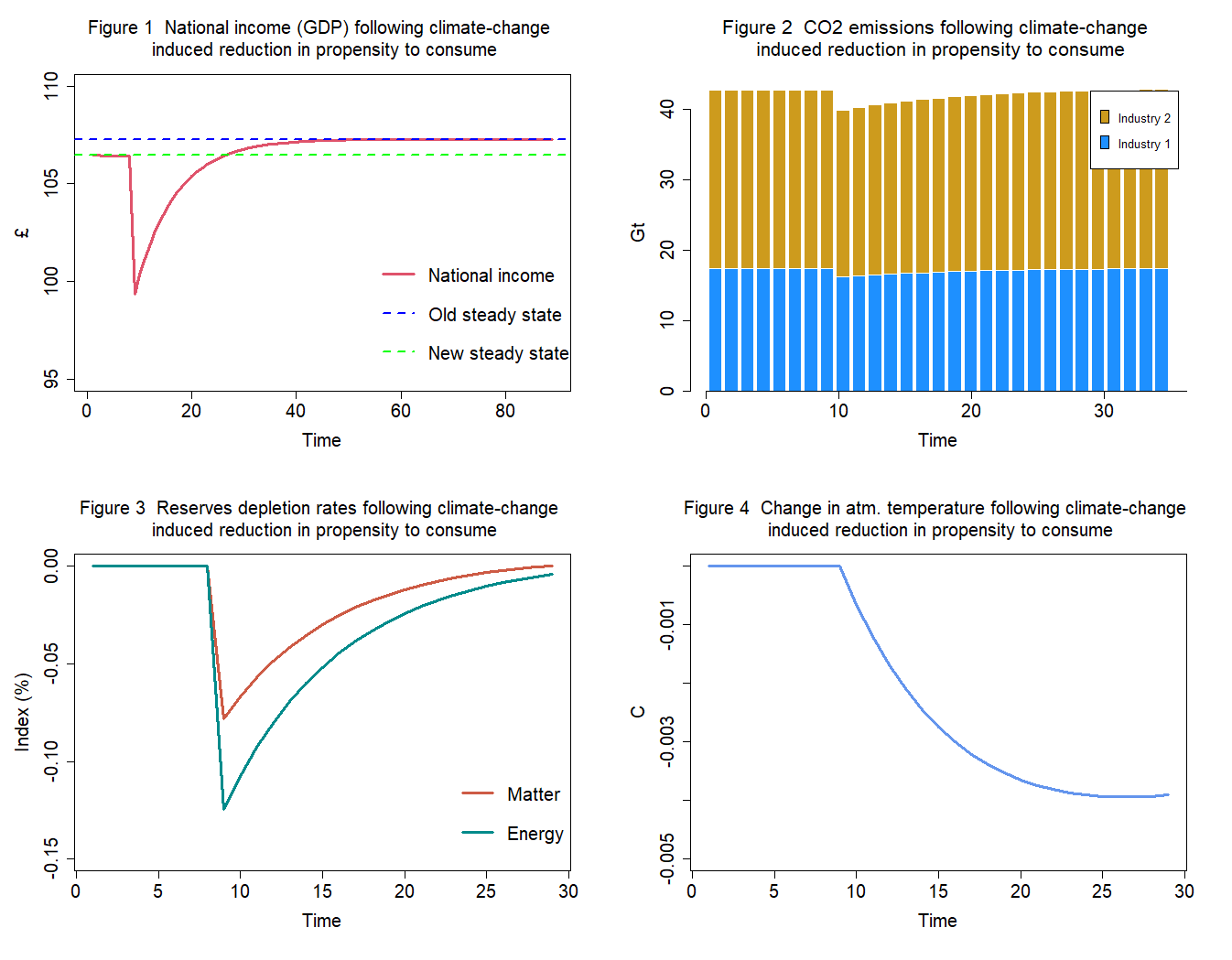
Lastly, feedback effects and damages can be introduced. Here the assumption is made that the propensity to consume out of income is (negatively) influenced by climate change.
#Endogenous propensity to consume out of income
alpha1[j,i] = a0[j,i] - a1[j,i] * (temp[j,i] - temp[j,i-1])
Now we can use the model to perform some experiments. For instance, we may want to examine how key variables behave when the propensity to consume out of income is influenced by an industrial CO2 emissions-led increase in atmospheric temperature:
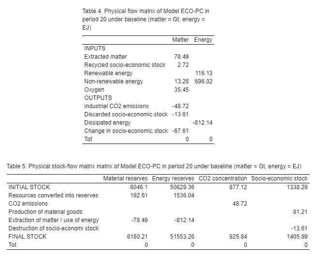
Notice that model identities for the ecosystem are derived from a physical flow matrix and a physical stock-flow matrix. The latter are automatically generated by this supplementary code.
Empirical SFC Models are SFC models whose coefficients are calibrated or estimated based on observed data. They are usually developed for studying national economies. There are two branches of Empirical SFC models:
-
Type I or data-to-theory models: these models are tailored to the country-specific sectoral balance sheets and flow of funds statistics of the economy under investigation (please refer to Zezza 2019).
-
Type II or theory-to-data models: these models are developed based on a theoretical SFC model, and then data are collected and adequately reclassified to estimate the coefficients of the model (e.g., Canelli et al. 2022).
For the sake of simplicity, the second approach is chosen here. In general, the choice of the specific approach depends on the research question one aims to address. Type I models are the best option for economies characterised by a country-specific institutional structure. In contrast, type II models allow for the reduction of the model size, thereby making findings clearer (although arguably less accurate).
Bimets is a software framework for R designed for time series analysis and econometric modeling. It allows creating and manipulating time series, specifying simultaneous equation models, performing model estimation, structural stability analysis, deterministic and stochastic simulation, forecasting, and performing optimal control. It can be conveniently used to develop, estimate, and simulate empirical SFC models.
Model EMP has been developed by reclassifying Eurostat data for Italy (1995-2021) to align with Model PC equations. In contrast to previous models, EMP has been coded using a dedicated R package (Bimets). The model code is organised into five different files
The first file, named EMP_model.R, allows creating the system of difference equations, uploading the observed series, and estimating model coefficients. As usual, the first step is to prepare the workspace:
#Clear environment
rm(list=ls(all=TRUE))

#Clear plots
if(!is.null(dev.list())) dev.off()

#Clear console
cat("\014")
The next step is to upload data from a folder. This code takes the observed series from a Dropbox folder, containing Eurostat data for Italy over the period 1995-2021. Alternatively, one can download the data from here. Note that the observed series have been adequately reclassified to fit Model PC simplified structure (here is the original Excel file).
| Year | CONS* | INV | GOV | X | IM | Y | TAX* | WB | YD* | Hh | Hs* | Bs* | Bh* | NVh* | Rb | Bcb* |
|---|---|---|---|---|---|---|---|---|---|---|---|---|---|---|---|---|
| 1995 | 815945 | 198068 | 172298 | 243824 | 207651 | 988243 | 212456 | 353786 | 839948 | 42951 | 42951 | 507396 | 464445 | 507396 | 0.086177341 | 42951 |
| 1996 | 861627 | 202429 | 184246 | 247921 | 200535 | 1045873 | 217179.527 | 378499 | 868718.1081 | 43739 | 43739 | 514487.1081 | 470748.1081 | 514487.1081 | 0.091749554 | 43739 |
| 1997 | 899199 | 213028 | 193160 | 263802 | 223262 | 1092359 | 227109.9858 | 397066 | 908439.9432 | 46923 | 46923 | 523728.0513 | 476805.0513 | 523728.0513 | 0.075787064 | 46923 |
| 1998 | 939233 | 224747 | 199624 | 274042 | 239497 | 1138857 | 234998.531 | 395312 | 939994.1239 | 50305 | 50305 | 524489.1752 | 474184.1752 | 524489.1752 | 0.066758091 | 50305 |
| 1999 | 968945 | 237770 | 206206 | 272643 | 251716 | 1175151 | 241361.3261 | 410340 | 965445.3043 | 56333 | 56333 | 520989.4795 | 464656.4795 | 520989.4795 | 0.055196262 | 56333 |
| 2000 | 1021318 | 259037 | 220195 | 318172 | 307621 | 1241513 | 253432.0602 | 427487 | 1013728.241 | 59394 | 59394 | 513399.7201 | 454005.7201 | 513399.7201 | 0.054511407 | 59394 |
| 2001 | 1064179 | 271825 | 239959 | 334498 | 318022 | 1304138 | 265777.2981 | 451041 | 1063109.192 | 49167 | 49167 | 512329.9126 | 463162.9126 | 512329.9126 | 0.055538922 | 49167 |
| 2002 | 1099840 | 291267 | 250419 | 329564 | 319342 | 1350259 | 275196.5138 | 470108 | 1100786.055 | 53408 | 53408 | 513275.9677 | 459867.9677 | 513275.9677 | 0.04940057 | 53408 |
| 2003 | 1130044 | 295388 | 264649 | 324994 | 318642 | 1394693 | 283482.1479 | 490889 | 1133928.592 | 64267 | 64267 | 517160.5595 | 452893.5595 | 517160.5595 | 0.046025005 | 64267 |
| 2004 | 1174064 | 308799 | 278255 | 348699 | 340141 | 1452319 | 294632.6857 | 509540 | 1178530.743 | 76070 | 76070 | 521627.3021 | 445557.3021 | 521627.3021 | 0.043894897 | 76070 |
| 2005 | 1200666 | 316194 | 292969 | 367451 | 368928 | 1493635 | 302638.5384 | 531929 | 1210554.154 | 89146 | 89146 | 531515.4557 | 442369.4557 | 531515.4557 | 0.042261228 | 89146 |
| 2006 | 1250165 | 340933 | 302522 | 406392 | 419143 | 1552687 | 314276.4153 | 555830 | 1257105.661 | 103968 | 103968 | 538456.1168 | 434488.1168 | 538456.1168 | 0.041212401 | 103968 |
| 2007 | 1307574 | 359238 | 307266 | 441837 | 447317 | 1614840 | 326549.2597 | 576340 | 1306197.039 | 112983 | 112983 | 537079.1556 | 424096.1556 | 537079.1556 | 0.044067272 | 112983 |
| 2008 | 1317366 | 356666 | 320333 | 439932 | 452498 | 1637699 | 331277.5521 | 595572 | 1325110.209 | 123257 | 123257 | 544823.3641 | 421566.3641 | 544823.3641 | 0.045706963 | 123257 |
| 2009 | 1251101 | 307703 | 326155 | 353292 | 363078 | 1577256 | 319304.9036 | 590431 | 1277219.615 | 129192 | 129192 | 570941.9787 | 441749.9787 | 570941.9787 | 0.038157551 | 129192 |
| 2010 | 1280114 | 331599 | 331166 | 404013 | 433952 | 1611280 | 325627.2195 | 599034 | 1302508.878 | 133437 | 133437 | 593336.8565 | 459899.8565 | 593336.8565 | 0.036033224 | 133437 |
| 2011 | 1322039 | 337468 | 326718 | 443061 | 466151 | 1648757 | 333065.7349 | 608088 | 1332262.94 | 141838 | 141838 | 603560.7962 | 461722.7962 | 603560.7962 | 0.038114264 | 141838 |
| 2012 | 1302605 | 288966 | 321754 | 460981 | 443052 | 1624359 | 328391.4449 | 600264 | 1313565.78 | 137756 | 137756 | 614521.5758 | 476765.5758 | 614521.5758 | 0.040955894 | 137756 |
| 2013 | 1293311 | 272433 | 319441 | 461783 | 423095 | 1612752 | 326455.6721 | 594339 | 1305822.688 | 139992 | 139992 | 627033.2641 | 487041.2641 | 627033.2641 | 0.036395019 | 139992 |
| 2014 | 1309427 | 275995 | 317979 | 473719 | 426597 | 1627406 | 329026.3752 | 595991 | 1316105.501 | 141353 | 141353 | 633711.765 | 492358.765 | 633711.765 | 0.033408732 | 141353 |
| 2015 | 1339011 | 283186 | 316344 | 491905 | 442016 | 1655355 | 334360.8164 | 609506 | 1337443.266 | 144595 | 144595 | 632144.0306 | 487549.0306 | 632144.0306 | 0.029554695 | 144595 |
| 2016 | 1373138 | 297798 | 322650 | 497339 | 441578 | 1695788 | 342039.4726 | 625000 | 1368157.89 | 150624 | 150624 | 627163.9209 | 476539.9209 | 627163.9209 | 0.028319924 | 150624 |
| 2017 | 1409591 | 313526 | 327002 | 533720 | 483997 | 1736593 | 350017.7149 | 642230 | 1400070.859 | 155752 | 155752 | 617643.7804 | 461891.7804 | 617643.7804 | 0.027309766 | 155752 |
| 2018 | 1436937 | 328194 | 334454 | 555394 | 512818 | 1771391 | 356801.0313 | 665490 | 1427204.125 | 162421 | 162421 | 607910.9055 | 445489.9055 | 607910.9055 | 0.026346512 | 162421 |
| 2019 | 1462136 | 327703 | 334512 | 567784 | 508031 | 1796648 | 361677.021 | 681104 | 1446708.084 | 165890 | 165890 | 592482.9897 | 426592.9897 | 592482.9897 | 0.023887824 | 165890 |
| 2020 | 1317041 | 293530 | 343580 | 488941 | 429156 | 1660621 | 334162.2757 | 642972 | 1336649.103 | 185433 | 185433 | 612091.0923 | 426658.0923 | 612091.0923 | 0.022529526 | 185433 |
| 2021 | 1429333 | 357215 | 352718 | 582192 | 540198 | 1782051 | 358332.6809 | 692915 | 1433330.724 | 200683 | 200683 | 616088.8159 | 415405.8159 | 616088.8159 | 0.023582902 | 200683 |
where * means that the series has been recalculated or reclassified to be coherent with Model PC aggregation level and/or fit model identities.
Once the data have been downloaded and re-organised, we can load them into the main code, along with the necessary R libraries.
#Upload libraries
library(bimets)
library(knitr)

#Upload data: time series for transactions-flow matrix and balance sheet from Dropbox
Data_PC <- read.csv("https://www.dropbox.com/scl/fi/ei74ev9i5yx91qwu9xz5f/PC_data.csv?rlkey=5t0leh5zxwqq2m07va8brq9yc&dl=1")

#Alternatively, upload data from your folder
#Data_PC <- read.csv("C:/.../PC_data.csv")
We can now define the system of identities and behavioural equations as a ".txt" file. Bimets syntax is quite intuitive. The reference manual can be found here.
S_model.txt="MODEL

COMMENT> GDP - eq. 4.1
IDENTITY> y
EQ> y = cons + g

COMMENT> Disposable income - eq. 4.2
IDENTITY> yd
EQ> yd = y - t + TSLAG(r,1)*TSLAG(b_h,1)

COMMENT> Tax revenues - eq. 4.3
BEHAVIORAL> t
TSRANGE 1998 1 2021 1
EQ> t = theta*(TSLAG(y,1) + TSLAG(r,1)*TSLAG(b_h,1))
COEFF> theta

COMMENT> Wealth accumulation - eq. 4.4
IDENTITY> v
EQ> v = TSLAG(v,1) + (yd - cons)

COMMENT> Household consumption - eq. 4.5
BEHAVIORAL> cons
TSRANGE 1998 1 2021 1
EQ> cons = alpha1*TSLAG(yd,1) + alpha2*TSLAG(v,1)
COEFF> alpha1 alpha2

COMMENT> Cash money - eq. 4.6
IDENTITY> h_h
EQ> h_h = v - b_h

COMMENT> Demand for government bills - eq. 4.7
BEHAVIORAL> b_h
TSRANGE 1998 1 2021 1
EQ> b_h = lambda0*v + lambda1*r*v + lambda2*yd
COEFF> lambda0 lambda1 lambda2

COMMENT> Supply of government bills - eq. 4.8
IDENTITY> b_s
EQ> b_s = TSLAG(b_s,1) + (g + TSLAG(r,1)*TSLAG(b_s,1)) - (t + TSLAG(r,1)*TSLAG(b_cb,1))

COMMENT> Supply of cash - eq. 4.9
IDENTITY> h_s
EQ> h_s = TSLAG(h_s,1) + b_cb - TSLAG(b_cb,1)

COMMENT> Government bills held by the central bank - eq. 4.10
IDENTITY> b_cb
EQ> b_cb = b_s - b_h

COMMENT> Interest rate as policy instrument - eq. 4.11
BEHAVIORAL> r
TSRANGE 1998 1 2021 1
EQ> r = par0 + par1*TSLAG(r,1)
COEFF> par0 par1

END"
The next step is to upload the observed series into the model.
#Load the model
PC_model=LOAD_MODEL(modelText = S_model.txt)

#Attribute values to model variables and coefficients
PC_modelData=list(

  y = TIMESERIES(c(Data_PC$Y),START=c(1995,1),FREQ=1),

  cons = TIMESERIES(c(Data_PC$CONS),START=c(1995,1),FREQ=1),

  g = TIMESERIES(c(Data_PC$GOV),START=c(1995,1),FREQ=1),

  yd = TIMESERIES(c(Data_PC$YD),START=c(1995,1),FREQ=1),

  t = TIMESERIES(c(Data_PC$TAX),START=c(1995,1),FREQ=1),

  r = TIMESERIES(c(Data_PC$Rb),START=c(1995,1),FREQ=1),

  r_bar = TIMESERIES(c(Data_PC$Rb),START=c(1995,1),FREQ=1),

  b_h = TIMESERIES(c(Data_PC$Bh),START=c(1995,1),FREQ=1),

  b_s = TIMESERIES(c(Data_PC$Bs),START=c(1995,1),FREQ=1),

  b_cb = TIMESERIES(c(Data_PC$Bcb),START=c(1995,1),FREQ=1),

  v = TIMESERIES(c(Data_PC$NVh ),START=c(1995,1),FREQ=1),

  h_h = TIMESERIES(c(Data_PC$Hh),START=c(1995,1),FREQ=1),

  h_s = TIMESERIES(c(Data_PC$Hs),START=c(1995,1),FREQ=1)

)

#Load the data into the model
PC_model=LOAD_MODEL_DATA(PC_model,PC_modelData)
We can now estimate model coefficients
#Estimate model coefficients
PC_model=ESTIMATE(PC_model
                 ,TSRANGE=c(1998,1,2019,1)            #Choose time range for estimations
                 #,forceTSRANGE = TRUE                 #Force same time range for all estimations
                 #,CHOWTEST = TRUE                     #Perform Chow test: stability analysis
)
When the CHOWTEST argument is set to TRUE, the model conducts a structural stability analysis to identify breaks.
The second file, named EMP_model_insample.R, performs in-sample predictions to check EMP's fit on actual data and enables the user to adjust predicted series to observed ones.
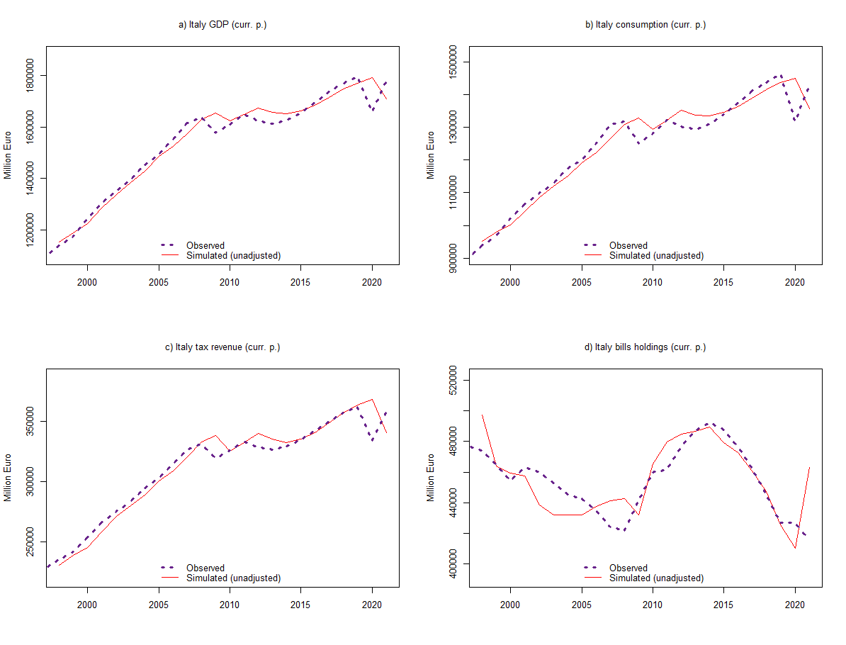
More precisely, the first step is to run the model to assess its fit with observed series. In this case, endogenous variables should not be exogenised, except for the policy tools (the policy rate, r, in this simplified model). Since we are conducting an in-sample simulation, we choose a static prediction approach, implying that historical values for the lagged endogenous variables are utilised in the solutions of subsequent periods.
# Define exogenisation list to 2021
exogenizeList <- list(  r = TRUE  )    #Interest rate

# In-sample prediction (no add factors)
PC_model <- SIMULATE(PC_model
                     ,simType='STATIC'
                     ,TSRANGE=c(1998,1,2021,1)
                     ,simConvergence=0.00001
                     ,simIterLimit=100
                     ,Exogenize=exogenizeList
                     ,quietly=TRUE)
We can now plot the simulated series against the observed series.
#PLOTS FOR VISUAL INSPECTION
layout(matrix(c(1:4), 2, 2, byrow = TRUE))

# GDP
plot(PC_model$simulation$y,col="red1",lty=1,lwd=1,font.main=1,cex.main=1,main="a) Italy GDP (thous. eur, curr. p.)",
     ylab = 'Million Euro',xlab = '', cex.axis=1,cex.lab=1,xlim=range(1998,2021),
     ylim=range(min(PC_model$simulation$y*0.95),max(PC_model$simulation$y*1.05)))
lines(PC_modelData$y,col="darkorchid4",lty=3,lwd=3)
legend("bottom",c("Observed","Simulated (unadjusted)"),  bty = "n", cex=1, lty=c(3,1), lwd=c(3,1),
       col = c("darkorchid4","red1"), box.lty=0)

# Consumption
plot(PC_model$simulation$cons,col="red1",lty=1,lwd=1,font.main=1,cex.main=1,main="b) Italy consumption (thous. eur, curr. p.)",
     ylab = 'Million Euro',xlab = '', cex.axis=1,cex.lab=1,xlim=range(1998,2021),
     ylim=range(min(PC_model$simulation$cons*0.95),max(PC_model$simulation$cons*1.05)))
lines(PC_modelData$cons,col="darkorchid4",lty=3,lwd=3)
legend("bottom",c("Observed","Simulated (unadjusted)"),  bty = "n", cex=1, lty=c(3,1), lwd=c(3,1),
       col = c("darkorchid4","red1"), box.lty=0)

# Tax revenue
plot(PC_model$simulation$t,col="red1",lty=1,lwd=1,font.main=1,cex.main=1,main="c) Italy tax revenue (thous. eur, curr. p.)",
     ylab = 'Million Euro',xlab = '', cex.axis=1,cex.lab=1,xlim=range(1998,2021),
     ylim=range(min(PC_model$simulation$t*0.95),max(PC_model$simulation$t*1.05)))
lines(PC_modelData$t,col="darkorchid4",lty=3,lwd=3)
legend("bottom",c("Observed","Simulated (unadjusted)"),  bty = "n", cex=1, lty=c(3,1), lwd=c(3,1),
       col = c("darkorchid4","red1"), box.lty=0)

# Bills held by househeolds
plot(PC_model$simulation$b_h,col="red1",lty=1,lwd=1,font.main=1,cex.main=1,main="d) Italy bills holdings (thous. eur, curr. p.)",
     ylab = 'Million Euro',xlab = '', cex.axis=1,cex.lab=1,xlim=range(1998,2021),
     ylim=range(min(PC_model$simulation$b_h*0.95),max(PC_model$simulation$b_h*1.05)))
lines(PC_modelData$b_h,col="darkorchid4",lty=3,lwd=3)
legend("bottom",c("Observed","Simulated (unadjusted)"),  bty = "n", cex=1, lty=c(3,1), lwd=c(3,1),
       col = c("darkorchid4","red1"), box.lty=0)
A consistency check, based on the redundant equation, can be conducted too (we refer to the complete code). After that, in-sample predictions can be adjusted to the observed series using prediction errors, that is, by exogenising the endogenous variables of the model.
# Define new exogenisation list to 2021
exogenizeList <- list(

  r = TRUE,                     #Interest rate
  t = TRUE,                     #Taxes
  cons = TRUE,                  #Consumption
  b_h = TRUE                    #Bills held by households

)

# Simulate model
PC_model <- SIMULATE(PC_model
                    ,simType='STATIC'
                    ,TSRANGE=c(1998,1,2021,1)
                    ,simConvergence=0.00001
                    ,simIterLimit=100
                    ,Exogenize=exogenizeList
                    ,quietly=TRUE)
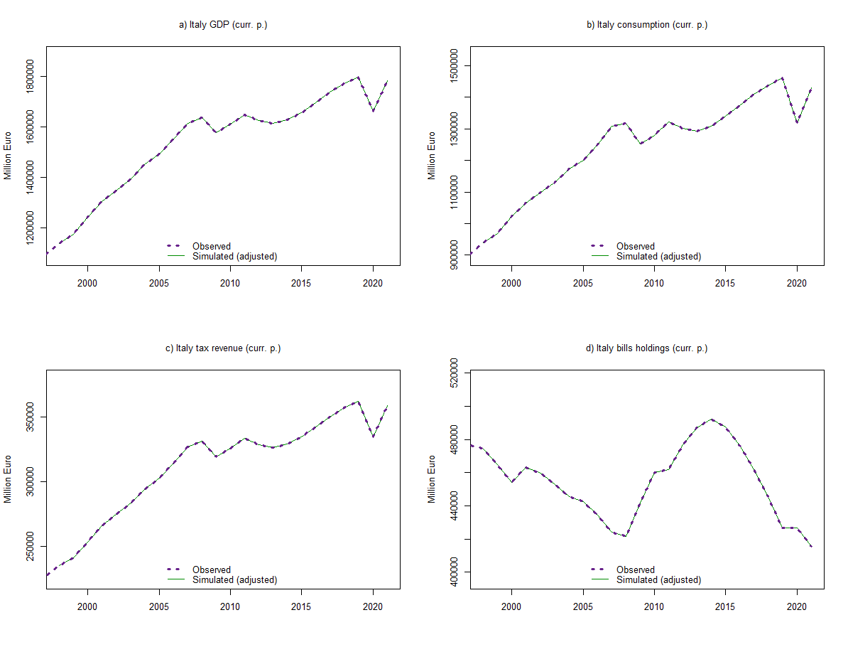
Simulated series now perfectly match observed ones over the considered period.
#PLOTS FOR VISUAL INSPECTION
layout(matrix(c(1:4), 2, 2, byrow = TRUE))

# GDP
plot(PC_model$simulation$y,col="green4",lty=1,lwd=1,font.main=1,cex.main=1,main="a) Italy GDP (curr. p.)",
     ylab = 'Million Euro',xlab = '', cex.axis=1,cex.lab=1,xlim=range(1998,2021),
     ylim=range(min(PC_model$simulation$y*0.95),max(PC_model$simulation$y*1.05)))
lines(PC_modelData$y,col="darkorchid4",lty=3,lwd=3)
legend("bottom",c("Observed","Simulated (adjusted)"),  bty = "n", cex=1, lty=c(3,1), lwd=c(3,1),
       col = c("darkorchid4","green4"), box.lty=0)

# Consumption
plot(PC_model$simulation$cons,col="green4",lty=1,lwd=1,font.main=1,cex.main=1,main="b) Italy consumption (curr. p.)",
     ylab = 'Million Euro',xlab = '', cex.axis=1,cex.lab=1,xlim=range(1998,2021),
     ylim=range(min(PC_model$simulation$cons*0.95),max(PC_model$simulation$cons*1.05)))
lines(PC_modelData$cons,col="darkorchid4",lty=3,lwd=3)
legend("bottom",c("Observed","Simulated (adjusted)"),  bty = "n", cex=1, lty=c(3,1), lwd=c(3,1),
       col = c("darkorchid4","green4"), box.lty=0)

# Tax revenue
plot(PC_model$simulation$t,col="green4",lty=1,lwd=1,font.main=1,cex.main=1,main="c) Italy tax revenue (curr. p.)",
     ylab = 'Million Euro',xlab = '', cex.axis=1,cex.lab=1,xlim=range(1998,2021),
     ylim=range(min(PC_model$simulation$t*0.95),max(PC_model$simulation$t*1.05)))
lines(PC_modelData$t,col="darkorchid4",lty=3,lwd=3)
legend("bottom",c("Observed","Simulated (adjusted)"),  bty = "n", cex=1, lty=c(3,1), lwd=c(3,1),
       col = c("darkorchid4","green4"), box.lty=0)

# Bills held by households
plot(PC_model$simulation$b_h,col="green4",lty=1,lwd=1,font.main=1,cex.main=1,main="d) Italy bills holdings (curr. p.)",
     ylab = 'Million Euro',xlab = '', cex.axis=1,cex.lab=1,xlim=range(1998,2021),
     ylim=range(min(PC_model$simulation$b_h*0.95),max(PC_model$simulation$b_h*1.05)))
lines(PC_modelData$b_h,col="darkorchid4",lty=3,lwd=3)
legend("bottom",c("Observed","Simulated (adjusted)"),  bty = "n", cex=1, lty=c(3,1), lwd=c(3,1),
col = c("darkorchid4","green4"), box.lty=0)The third file, named EMP_model_outofsample.R, performs out-of-sample predictions, of both deterministic and stochastic nature, which can be used as the baseline scenario.
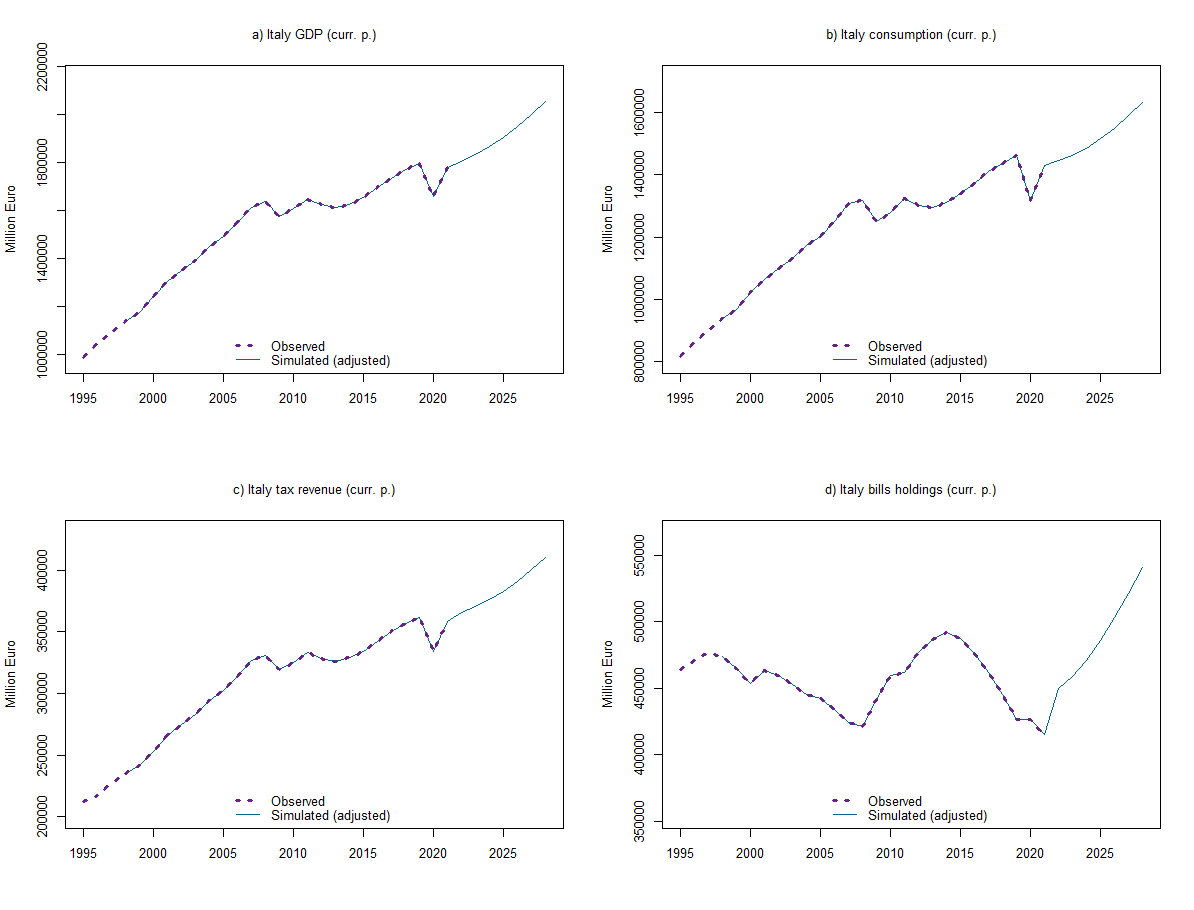
The first step is to extend exogenous variables up to the end of the forecasting period, which, in this exercise, is 2028. Similar to what we did for adjusted in-sample predictions, the second step is to create an "exogenization list", encompassing all the endogenous variables of the model. These variables are adjusted up to 2021 and then set free to follow the dynamics implied by the model equations.
Afterward, we can simulate the model out of sample using either the function DYNAMIC (employing simulated values for the lagged endogenous variables in the solutions of subsequent periods) or the function FORECAST (similar to the previous one, but setting the starting values of endogenous variables in a period equal to the simulated values of the previous period).
# Extend exogenous and conditionally-evaluated variables up to 2028
PC_model$modelData <- within(PC_model$modelData,{ g = TSEXTEND(g,  UPTO=c(2028,1)) })

# Define exogenisation list
exogenizeList <- list(

  r = TRUE,                     #Interest rate (whole period)
  t = c(1998,1,2021,1),         #Taxes
  cons = c(1998,1,2021,1),      #Consumption
  b_h = c(1998,1,2021,1)        #Bills held by households

)

# Simulate model
PC_model <- SIMULATE(PC_model
                    ,simType='DYNAMIC' #try also: 'FORECAST'
                    ,TSRANGE=c(1998,1,2028,1)
                    ,simConvergence=0.00001
                    ,simIterLimit=1000
                    ,Exogenize=exogenizeList
                    #,ConstantAdjustment=constantAdjList
                    ,quietly=TRUE)

#PLOTS FOR VISUAL INSPECTION
layout(matrix(c(1:4), 2, 2, byrow = TRUE))

# GDP
plot(PC_model$simulation$y,col="deepskyblue4",lty=1,lwd=1,font.main=1,cex.main=1,main="a) Italy GDP (curr. p.)",
     ylab = 'Million Euro',xlab = '', cex.axis=1,cex.lab=1,xlim=range(1995,2028),
     ylim=range(min(PC_model$simulation$y*0.85),max(PC_model$simulation$y*1.05)))
lines(PC_modelData$y,col="darkorchid4",lty=3,lwd=3)
legend("bottom",c("Observed","Simulated (adjusted)"),  bty = "n", cex=1, lty=c(3,1), lwd=c(3,1),
       col = c("darkorchid4","deepskyblue4"), box.lty=0)

# Consumption
plot(PC_model$simulation$cons,col="deepskyblue4",lty=1,lwd=1,font.main=1,cex.main=1,main="b) Italy consumption (curr. p.)",
     ylab = 'Million Euro',xlab = '', cex.axis=1,cex.lab=1,xlim=range(1995,2028),
     ylim=range(min(PC_model$simulation$cons*0.85),max(PC_model$simulation$cons*1.05)))
lines(PC_modelData$cons,col="darkorchid4",lty=3,lwd=3)
legend("bottom",c("Observed","Simulated (adjusted)"),  bty = "n", cex=1, lty=c(3,1), lwd=c(3,1),
       col = c("darkorchid4","deepskyblue4"), box.lty=0)

# Tax revenue
plot(PC_model$simulation$t,col="deepskyblue4",lty=1,lwd=1,font.main=1,cex.main=1,main="c) Italy tax revenue (curr. p.)",
     ylab = 'Million Euro',xlab = '', cex.axis=1,cex.lab=1,xlim=range(1995,2028),
     ylim=range(min(PC_model$simulation$t*0.85),max(PC_model$simulation$t*1.05)))
lines(PC_modelData$t,col="darkorchid4",lty=3,lwd=3)
legend("bottom",c("Observed","Simulated (adjusted)"),  bty = "n", cex=1, lty=c(3,1), lwd=c(3,1),
       col = c("darkorchid4","deepskyblue4"), box.lty=0)

# Bills held by househeolds
plot(PC_model$simulation$b_h,col="deepskyblue4",lty=1,lwd=1,font.main=1,cex.main=1,main="d) Italy bills holdings (curr. p.)",
     ylab = 'Million Euro',xlab = '', cex.axis=1,cex.lab=1,xlim=range(1995,2028),
     ylim=range(min(PC_model$simulation$b_h*0.85),max(PC_model$simulation$b_h*1.05)))
lines(PC_modelData$b_h,col="darkorchid4",lty=3,lwd=3)
legend("bottom",c("Observed","Simulated (adjusted)"),  bty = "n", cex=1, lty=c(3,1), lwd=c(3,1),
       col = c("darkorchid4","deepskyblue4"), box.lty=0)
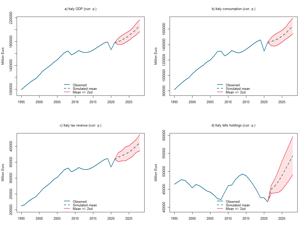
The simulations above are deterministic in nature. However, Bimets also allows conducting stochastic simulations using the STOCHSIMULATE function. This enables the analysis of forecast errors in structural econometric models arising from random disturbances, coefficient estimation errors, etc. More precisely, the model is solved for different values of specified stochastic disturbances, the structure of which is defined by users, specifying probability distributions and time ranges. Mean and standard deviation for each simulated endogenous variable are stored in the output model object.
#Define stochastic structure (disturbances)
myStochStructure <- list(

  #Consumption: normally-distributed shocks
  cons=list(
    TSRANGE=c(2022,1,2028,1),
    TYPE='NORM', #UNIF
    PARS=c(0,PC_model$behaviorals$cons$statistics$StandardErrorRegression)
  ),

  #Taxes: normally-distributed shocks
  t=list(
    TSRANGE=c(2022,1,2028,1),
    TYPE='NORM', #UNIF
    PARS=c(0,PC_model$behaviorals$t$statistics$StandardErrorRegression)
  )

)

# Simulate model again
PC_model <- STOCHSIMULATE(PC_model
                         ,simType='FORECAST'
                         ,TSRANGE=c(2021,1,2028,1)
                         ,StochStructure=myStochStructure
                         ,StochSeed=123
                         ,simConvergence=0.00001
                         ,simIterLimit=1000
                         ,Exogenize=exogenizeList
                         ,ConstantAdjustment=constantAdjList
                         ,quietly=TRUE)
It is important to stress that two types of shocks for the stochastic structure of the model can be selected. NORM stands for "normal distribution." In this case, parameters must contain the mean and the standard deviation of the normal distribution. UNIF stands for "uniform distribution." The related parameters must contain the lower and upper bounds of the uniform distribution.
Having specified that, we can now re-plot the charts.
#Set layout
layout(matrix(c(1:4), 2, 2, byrow = TRUE))

#Create custom colours
mycol1 <- rgb(0,255,0, max = 255, alpha = 80)
mycol2 <- rgb(255,0,0, max = 255, alpha = 30)

#Create and dsplay the charts

# GDP
plot(PC_model$stochastic_simulation$y$mean,col="deepskyblue4",lty=2,lwd=2,font.main=1,cex.main=1,
     main="a) Italy GDP (curr. p.)",
     ylab = 'Million Euro',xlab = '', cex.axis=1,cex.lab=1,xlim=range(1995,2028),
     ylim=range(min(PC_modelData$y*0.95),max(PC_model$stochastic_simulation$y$mean*1.05)))
lines(PC_model$stochastic_simulation$y$mean+2*PC_model$stochastic_simulation$y$sd,col=2,lty=1,lwd=2)
lines(PC_model$stochastic_simulation$y$mean-2*PC_model$stochastic_simulation$y$sd,col=2,lty=1,lwd=2)
lines(PC_modelData$y,col="deepskyblue4",lty=1,lwd=2)
x_values <- seq(2021, 2028)
y_upper <- PC_model$stochastic_simulation$y$mean + 2 * PC_model$stochastic_simulation$y$sd
y_lower <- PC_model$stochastic_simulation$y$mean - 2 * PC_model$stochastic_simulation$y$sd
polygon(
  c(x_values, rev(x_values)),
  c(y_upper, rev(y_lower)),
  col = mycol2,
  border = NA )
legend("bottom",c("Observed","Simulated mean","Mean +/- 2sd"),  bty = "n", cex=1,
       lty=c(1,2,1), lwd=c(2,2,2), col = c("deepskyblue4","deepskyblue4",2), box.lty=0)

# Consumption
plot(PC_model$stochastic_simulation$cons$mean,col="deepskyblue4",lty=2,lwd=2,font.main=1,cex.main=1,
     main="b) Italy consumption (curr. p.)",
     ylab = 'Million Euro',xlab = '', cex.axis=1,cex.lab=1,xlim=range(1995,2028),
     ylim=range(min(PC_modelData$cons*0.95),max(PC_model$stochastic_simulation$cons$mean*1.05)))
lines(PC_model$stochastic_simulation$cons$mean+2*PC_model$stochastic_simulation$cons$sd,col=2,lty=1,lwd=2)
lines(PC_model$stochastic_simulation$cons$mean-2*PC_model$stochastic_simulation$cons$sd,col=2,lty=1,lwd=2)
lines(PC_modelData$cons,col="deepskyblue4",lty=1,lwd=2)
x_values <- seq(2021, 2028)
y_upper <- PC_model$stochastic_simulation$cons$mean + 2 * PC_model$stochastic_simulation$cons$sd
y_lower <- PC_model$stochastic_simulation$cons$mean - 2 * PC_model$stochastic_simulation$cons$sd
polygon(
  c(x_values, rev(x_values)),
  c(y_upper, rev(y_lower)),
  col = mycol2,
  border = NA )
legend("bottom",c("Observed","Simulated mean","Mean +/- 2sd"),  bty = "n", cex=1,
       lty=c(1,2,1), lwd=c(2,2,2), col = c("deepskyblue4","deepskyblue4",2), box.lty=0)

# Tax revenue
plot(PC_model$stochastic_simulation$t$mean,col="deepskyblue4",lty=2,lwd=2,font.main=1,cex.main=1,
     main="c) Italy tax revenue (curr. p.)",
     ylab = 'Million Euro',xlab = '', cex.axis=1,cex.lab=1,xlim=range(1995,2028),
     ylim=range(min(PC_modelData$t*0.95),max(PC_model$stochastic_simulation$t$mean*1.05)))
lines(PC_model$stochastic_simulation$t$mean+2*PC_model$stochastic_simulation$t$sd,col=2,lty=1,lwd=2)
lines(PC_model$stochastic_simulation$t$mean-2*PC_model$stochastic_simulation$t$sd,col=2,lty=1,lwd=2)
lines(PC_modelData$t,col="deepskyblue4",lty=1,lwd=2)
x_values <- seq(2021, 2028)
y_upper <- PC_model$stochastic_simulation$t$mean + 2 * PC_model$stochastic_simulation$t$sd
y_lower <- PC_model$stochastic_simulation$t$mean - 2 * PC_model$stochastic_simulation$t$sd
polygon(
  c(x_values, rev(x_values)),
  c(y_upper, rev(y_lower)),
  col = mycol2,
  border = NA )
legend("bottom",c("Observed","Simulated mean","Mean +/- 2sd"),  bty = "n", cex=1,
       lty=c(1,2,1), lwd=c(2,2,2), col = c("deepskyblue4","deepskyblue4",2), box.lty=0)

# Bills held by households
plot(PC_model$stochastic_simulation$b_h$mean,col="deepskyblue4",lty=2,lwd=2,font.main=1,cex.main=1,
     main="d) Italy bills holdings (curr. p.)",
     ylab = 'Million Euro',xlab = '', cex.axis=1,cex.lab=1,xlim=range(1995,2028),
     ylim=range(min(PC_modelData$b_h*0.95),max(PC_model$stochastic_simulation$b_h$mean*1.1)))
lines(PC_model$stochastic_simulation$b_h$mean+2*PC_model$stochastic_simulation$b_h$sd,col=2,lty=1,lwd=2)
lines(PC_model$stochastic_simulation$b_h$mean-2*PC_model$stochastic_simulation$b_h$sd,col=2,lty=1,lwd=2)
lines(PC_modelData$b_h,col="deepskyblue4",lty=1,lwd=2)
x_values <- seq(2021, 2028)
y_upper <- PC_model$stochastic_simulation$b_h$mean + 2 * PC_model$stochastic_simulation$b_h$sd
y_lower <- PC_model$stochastic_simulation$b_h$mean - 2 * PC_model$stochastic_simulation$b_h$sd
polygon(
  c(x_values, rev(x_values)),
  c(y_upper, rev(y_lower)),
  col = mycol2,
  border = NA )
legend("bottom",c("Observed","Simulated mean","Mean +/- 2sd"),  bty = "n", cex=1,
lty=c(1,2,1), lwd=c(2,2,2), col = c("deepskyblue4","deepskyblue4",2), box.lty=0)The fourth file, named EMP_model_tables.R, allows creating the balance sheet and the transactions-flow matrix of the economy, using either observed series or predicted ones.
Both the knitr and kableExtra packages are required. However, we highly recommend loading the latter after the tables have been created.
We start with the balance-sheet matrix.
#Create BS and TFM tables using observed time series

#Upload libraries
library(knitr)

#Choose a year - NOTE: 27 = 2021
yr=27

#Choose a scenario (note: 1 = baseline)
#scen=1

#Create row names for BS matrix
rownames<-c( "Cash (money)",
             "Bills",
             "Wealth",
             "Column total")

#Create households aggregates
H <-c( round(PC_modelData$h_h[yr], digits = 2),
       round(PC_modelData$b_h[yr], digits = 2),
       round(-PC_modelData$v[yr], digits = 2),
       round(-PC_modelData$v[yr]+PC_modelData$h_h[yr]+PC_modelData$b_h[yr], digits = 2)
)

#Create table of results
H_BS<-as.data.frame(H,row.names=rownames)

#Print firms column
kable(H_BS)

#Create firms aggregates
P <-c( "",
       "",
       "",
       0
)

#Create table of results
F_BS<-as.data.frame(P,row.names=rownames)

#Print firms column
kable(F_BS)

#Create government aggregates
G   <-c( "",
         round(-PC_modelData$b_s[yr], digits = 2),
         round(PC_modelData$b_s[yr], digits = 2),
         "0"
)

#Create table of results
G_BS<-as.data.frame(G,row.names=rownames)

#Print government column
kable(G_BS)

#Create CB aggregates
CB  <-c( round(-PC_modelData$h_s[yr], digits = 2),
         round(PC_modelData$b_cb[yr], digits = 2),
         "0",
         round(-PC_modelData$h_s[yr]+PC_modelData$b_cb[yr], digits = 2)
)

#Create table of results
CB_BS<-as.data.frame(CB,row.names=rownames)

#Print CB column
kable(CB_BS)

#Create "row total" column
Tot  <-c( round(PC_modelData$h_h[yr]-PC_modelData$h_s[yr], digits = 2),
          round(PC_modelData$b_h[yr]+PC_modelData$b_cb[yr]-PC_modelData$b_s[yr], digits = 2),
          round(-PC_modelData$v[yr]+PC_modelData$b_s[yr], digits = 2),
          round(PC_modelData$h_h[yr]-PC_modelData$h_s[yr]+
                  PC_modelData$b_h[yr]+PC_modelData$b_cb[yr]-PC_modelData$b_s[yr]+
                -PC_modelData$v[yr]+PC_modelData$b_s[yr], digits = 2)
)

#Create table of results
Tot_BS<-as.data.frame(Tot,row.names=rownames)

#Print total column
kable(Tot_BS)

#Create BS matrix
BS_Matrix<-cbind(H_BS,F_BS,CB_BS,G_BS,Tot_BS)
kable(BS_Matrix) #Unload kableExtra to use this
The commands above allow visualising the BS matrix in the console. However, an HTML version and a LaTeX version of the table can be generated too by adding the following commands.
#Upload libraries
library(kableExtra)

#Create captions
caption1 <- paste("Table 1. Balance sheet of Model EMP for Italy in ", yr+1994, "(curr. p.)")

#Create html table for BS
BS_Matrix %>%
  kbl(caption=caption1,
      format= "html",
      #format= "latex",
      col.names = c("Households","Firms","Central bank","Government","Row total"),
      align="r") %>%
  kable_classic(full_width = F, html_font = "helvetica")
We can now move to the transactions-flow matrix.
#Create row names for TFM
rownames<-c( "Consumption",
             "Government expenditure",
             "GDP (income)",
             "Interest payments",
             "CB profit",
             "Taxes",
             "Change in cash",
             "Change in bills",
             "Column total")

#Create households aggregates
H <-c( round(-PC_modelData$cons[yr], digits = 2),
       "",
       round(PC_modelData$y[yr], digits = 2),
       round(PC_modelData$r[yr-1]*PC_modelData$b_h[yr-1], digits = 2),
       "",
       round(-PC_modelData$t[yr], digits = 2),
       round(-PC_modelData$h_h[yr]+PC_modelData$h_h[yr-1], digits = 2),
       round(-PC_modelData$b_h[yr]+PC_modelData$b_h[yr-1], digits = 2),
       round(-PC_modelData$cons[yr]+PC_modelData$y[yr]+PC_modelData$r[yr-1]*PC_modelData$b_h[yr-1]-PC_modelData$t[yr]+
              -PC_modelData$h_h[yr]+PC_modelData$h_h[yr-1]-PC_modelData$b_h[yr]+PC_modelData$b_h[yr-1], digits = 2)
)

#Create table of results
H_TFM<-as.data.frame(H,row.names=rownames)

#Print households column
kable(H_TFM)

#Create firms aggregates
P <-c( round(PC_modelData$cons[yr], digits = 2),
       round(PC_modelData$g[yr], digits = 2),
       round(-PC_modelData$y[yr], digits = 2),
       "",
       "",
       "",
       "",
       "",
       round(PC_modelData$cons[yr]+PC_modelData$g[yr]-PC_modelData$y[yr], digits = 2)
)

#Create table of results
F_TFM<-as.data.frame(P,row.names=rownames)

#Print firms column
kable(F_TFM)

#Create government aggregates
G   <-c( "",
         round(-PC_modelData$g[yr], digits = 2),
         "",
         round(-PC_modelData$r[yr-1]*PC_modelData$b_s[yr-1], digits = 2),
         round(PC_modelData$r[yr-1]*PC_modelData$b_cb[yr-1], digits = 2),
         round(PC_modelData$t[yr], digits = 2),
         "",
         round(PC_modelData$b_s[yr]-PC_modelData$b_s[yr-1], digits = 2),
         round(-PC_modelData$g[yr]+
               -PC_modelData$r[yr-1]*PC_modelData$b_s[yr-1]+
                PC_modelData$r[yr-1]*PC_modelData$b_cb[yr-1]+
                PC_modelData$t[yr]+
                 PC_modelData$b_s[yr]-PC_modelData$b_s[yr-1], digits = 2)
)

#Create table of results
G_TFM<-as.data.frame(G,row.names=rownames)

#Print government column
kable(G_TFM)

#Create CB aggregates
CB   <-c( "",
         "",
         "",
         round(PC_modelData$r[yr-1]*PC_modelData$b_cb[yr-1], digits = 2),
         round(-PC_modelData$r[yr-1]*PC_modelData$b_cb[yr-1], digits = 2),
         "",
         round(PC_modelData$h_s[yr]-PC_modelData$h_s[yr-1], digits = 2),
         round(-PC_modelData$b_cb[yr]+PC_modelData$b_cb[yr-1], digits = 2),
         round(PC_modelData$h_s[yr]-PC_modelData$h_s[yr-1]-PC_modelData$b_cb[yr]+PC_modelData$b_cb[yr-1], digits = 2)
)

#Create table of results
CB_TFM<-as.data.frame(CB,row.names=rownames)

#Print CB column
kable(CB_TFM)

#Create "row total" column
Tot   <-c(round(PC_modelData$cons[yr]-PC_modelData$cons[yr], digits = 2),
          round(PC_modelData$g[yr]-PC_modelData$g[yr], digits = 2),
          round(PC_modelData$y[yr]-PC_modelData$y[yr], digits = 2),
          round(PC_modelData$r[yr-1]*PC_modelData$b_h[yr-1]+PC_modelData$r[yr-1]*PC_modelData$b_cb[yr-1]-PC_modelData$r[yr-1]*PC_modelData$b_s[yr-1], digits = 2),
          round(PC_modelData$r[yr-1]*PC_modelData$b_cb[yr-1]-PC_modelData$r[yr-1]*PC_modelData$b_cb[yr-1], digits = 2),
          round(-PC_modelData$t[yr]+PC_modelData$t[yr], digits = 2),
          round(-PC_modelData$h_h[yr]+PC_modelData$h_h[yr-1]+PC_modelData$h_s[yr]-PC_modelData$h_s[yr-1], digits = 2),
          round(-PC_modelData$b_h[yr]+PC_modelData$b_h[yr-1]-PC_modelData$b_cb[yr]+PC_modelData$b_cb[yr-1]+PC_modelData$b_s[yr]-PC_modelData$b_s[yr-1], digits = 2),
          round(PC_modelData$cons[yr]-PC_modelData$cons[yr]+
                  PC_modelData$g[yr]-PC_modelData$g[yr]+
                  PC_modelData$y[yr]-PC_modelData$y[yr]+
                  PC_modelData$r[yr-1]*PC_modelData$b_h[yr-1]+PC_modelData$r[yr-1]*PC_modelData$b_cb[yr-1]-PC_modelData$r[yr-1]*PC_modelData$b_s[yr-1]+
                  PC_modelData$r[yr-1]*PC_modelData$b_cb[yr-1]-PC_modelData$r[yr-1]*PC_modelData$b_cb[yr-1]+
                  -PC_modelData$t[yr]+PC_modelData$t[yr]+
                  -PC_modelData$h_h[yr]+PC_modelData$h_h[yr-1]+PC_modelData$h_s[yr]-PC_modelData$h_s[yr-1]+
                  -PC_modelData$b_h[yr]+PC_modelData$b_h[yr-1]-PC_modelData$b_cb[yr]+PC_modelData$b_cb[yr-1]+PC_modelData$b_s[yr]-PC_modelData$b_s[yr-1], digits = 2)
)

#Create table of results
Tot_TFM<-as.data.frame(Tot,row.names=rownames)

#Print total column
kable(Tot_TFM)

#Create TFM matrix
TFM_Matrix<-cbind(H_TFM,F_TFM,CB_TFM,G_TFM,Tot_TFM)
kable(TFM_Matrix) #Unload kableExtra to use this
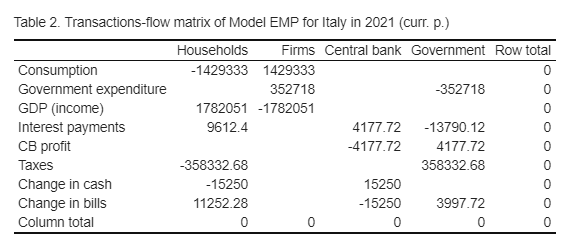
Once again, a htlm version (or a LaTeX version) of the table can be generated using kableExtra.
#Upload libraries
library(kableExtra)

#Create captions
caption2 <- paste("Table 2. Transactions-flow matrix of Model EMP for Italy in ",yr+1994, "(curr. p.)")

#Create html table for TFM
TFM_Matrix %>%
  kbl(caption=caption2,
      format= "html",
      #format= "latex",
      col.names = c("Households","Firms","Central bank","Government","Row total"),
      align="r") %>%
kable_classic(full_width = F, html_font = "helvetica")The fifth file, named EMP_model_sankey.R, generates the Sankey diagram of cross-sector transactions and changes in financial stocks. A few additional packages are required here.
#Upload libraries for Sankey diagram
library(networkD3)
library(htmlwidgets)
library(htmltools)

#Create nodes: source, target and flows
nodes = data.frame("name" =
                     c("Firms outflow", # Node 0
                       "Households outflow", # Node 1
                       "Government outflow", # Node 2

                       "Firms inflow", # Node 3
                       "Households inflow", # Node 4
                       "Government inflow", # Node 5

                       "Wages", # Node 6
                       "Consumption", # Node 7
                       "Taxes", # Node 8
                       "Government spending", # Node 9
                       "Money (change)", # Node 10

                       "Interest payments", # Node 11
                       "Bills (change)", # Node 12
                       "CB outflow", # Node 13
                       "CB inflow" # Node 14

                     ))

#Select a year - NOTE: 27 = 2021
yr=27

#Create the flows
links = as.data.frame(matrix(c(
  0, 6, PC_modelData$cons[yr]+PC_modelData$g[yr],
  1, 7, PC_modelData$cons[yr] ,
  1, 8, PC_modelData$t[yr],
  1, 10, PC_modelData$h_h[yr]-PC_modelData$h_h[yr-1],
  2, 9, PC_modelData$g[yr],
  6, 4, PC_modelData$cons[yr]+PC_modelData$g[yr],
  7, 3, PC_modelData$cons[yr],
  8, 5, PC_modelData$t[yr],
  9, 3, PC_modelData$g[yr],
  2, 11, PC_modelData$r[yr-1]*PC_modelData$b_h[yr-1],
  11, 4, PC_modelData$r[yr-1]*PC_modelData$b_h[yr-1],
  10, 14, PC_modelData$h_s[yr]-PC_modelData$h_s[yr-1],
  12, 5, PC_modelData$b_s[yr]-PC_modelData$b_s[yr-1],
  1, 12, PC_modelData$b_h[yr]-PC_modelData$b_h[yr-1],
  13, 12, PC_modelData$b_cb[yr]-PC_modelData$b_cb[yr-1]

),

#Note: each row represents a link. The first number represents the node being
#connected from. The second number represents the node connected to. The third
#number is the value of the node.

byrow = TRUE, ncol = 3))
names(links) = c("source", "target", "value")
my_color <- 'd3.scaleOrdinal() .domain([]) .range(["blue","green","yellow","red","purple","khaki","peru","violet","cyan","pink","orange","beige","white"])'

#Create and plot the network
sankeyNetwork(Links = links, Nodes = nodes,
              Source = "source", Target = "target",
              Value = "value", NodeID = "name", colourScale=my_color,
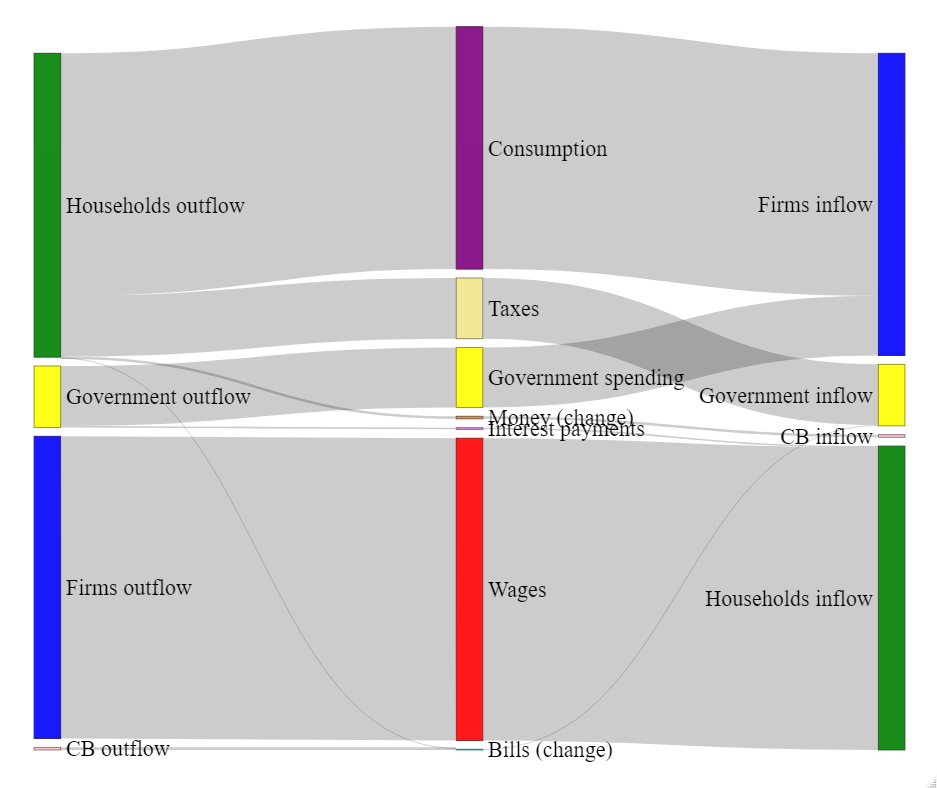
fontSize= 25, nodeWidth = 30)Tha last file, named EMP_model_experim.R, imposes exogenous shocks to selected model variables to create alternative scenarios (to be compared with the baseline scenario). Firstly, we rename the values of selected varaibles under the baseline scenario (deterministic out-of-sample simulations).
#Attribute values to selected variables
y_0=PC_model$simulation$y
cons_0=PC_model$simulation$cons
t_0=PC_model$simulation$t
b_h_0=PC_model$simulation$b_h
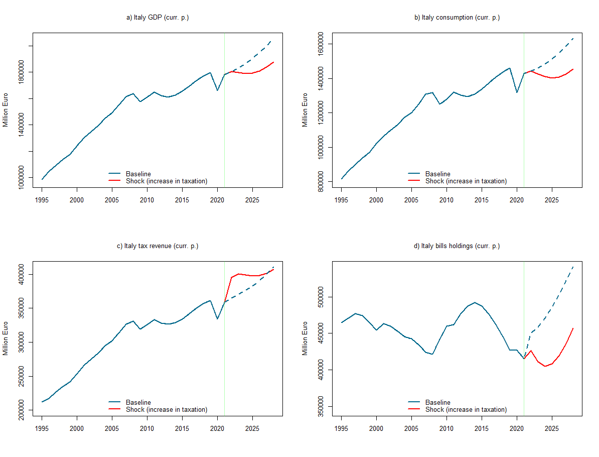
Secondly, we create one or more alternative scenarios by adding exogenous corrections to selected variables through the constantAdjList option and then re-run the model. More specifically, we test the effect of a fixed-sum increase in taxation amounting to 3 billion EUR.
# Extend exogenous and conditionally-evaluated variables up to 2028
PC_model$modelData <- within(PC_model$modelData,{ g = TSEXTEND(g,  UPTO=c(2028,1)) })

# Define exogenisation list
exogenizeList <- list(

  r = TRUE,                     #Interest rate (whole period)
  t = c(1998,1,2021,1),         #Taxes
  cons = c(1998,1,2021,1),      #Consumption
  b_h = c(1998,1,2021,1)        #Bills held by households

)

# Define add-factor list (defining exogenous adjustments: policy + available predictions)
constantAdjList <- list(

  cons = TIMESERIES(0,0,0,0,0,0,0,0,START=c(2021,1), FREQ='A'),  #Shock to consumption
  t    = TIMESERIES(30000,30000,30000,30000,30000,30000,30000,30000,START=c(2021,1), FREQ='A')  #Shock to taxes

)

# Simulate model
PC_model <- SIMULATE(PC_model
                     ,simType='DYNAMIC' #try also: 'FORECAST'
                     ,TSRANGE=c(1998,1,2028,1)
                     ,simConvergence=0.00001
                     ,simIterLimit=1000
                     ,Exogenize=exogenizeList
                     ,ConstantAdjustment=constantAdjList
                     ,quietly=TRUE)

#PLOTS FOR VISUAL INSPECTION

#Set layout
layout(matrix(c(1:4), 2, 2, byrow = TRUE))

#Create custom colours
mycol1 <- rgb(0,255,0, max = 255, alpha = 80)
mycol2 <- rgb(255,0,0, max = 255, alpha = 30)

# GDP
plot(PC_model$simulation$y,col="red1",lty=1,lwd=2,font.main=1,cex.main=1,main="a) Italy GDP (curr. p.)",
     ylab = 'Million Euro',xlab = '', cex.axis=1,cex.lab=1,xlim=range(1995,2028),
     ylim=range(min(PC_model$simulation$y*0.85),max(y_0)))
lines(y_0,col="deepskyblue4",lty=2,lwd=2)
lines(PC_modelData$y,col="deepskyblue4",lty=1,lwd=2)
abline(v=2021,col=mycol1)
legend("bottom",c("Baseline","Shock (increase in taxation)"),  bty = "n", cex=1, lty=c(1,1), lwd=c(2,2),
       col = c("deepskyblue4","red1"), box.lty=0)

# Consumption
plot(PC_model$simulation$cons,col="red1",lty=1,lwd=2,font.main=1,cex.main=1,main="b) Italy consumption (curr. p.)",
     ylab = 'Million Euro',xlab = '', cex.axis=1,cex.lab=1,xlim=range(1995,2028),
     ylim=range(min(PC_model$simulation$cons*0.85),max(cons_0)))
lines(cons_0,col="deepskyblue4",lty=2,lwd=2)
lines(PC_modelData$cons,col="deepskyblue4",lty=1,lwd=2)
abline(v=2021,col=mycol1)
legend("bottom",c("Baseline","Shock (increase in taxation)"),  bty = "n", cex=1, lty=c(1,1), lwd=c(2,2),
       col = c("deepskyblue4","red1"), box.lty=0)

# Tax revenue
plot(PC_model$simulation$t,col="red1",lty=1,lwd=2,font.main=1,cex.main=1,main="c) Italy tax revenue (curr. p.)",
     ylab = 'Million Euro',xlab = '', cex.axis=1,cex.lab=1,xlim=range(1995,2028),
     ylim=range(min(PC_model$simulation$t*0.85),max(t_0)))
lines(t_0,col="deepskyblue4",lty=2,lwd=2)
lines(PC_modelData$t,col="deepskyblue4",lty=1,lwd=2)
abline(v=2021,col=mycol1)
legend("bottom",c("Baseline","Shock (increase in taxation)"),  bty = "n", cex=1, lty=c(1,1), lwd=c(2,2),
       col = c("deepskyblue4","red1"), box.lty=0)

# Bills held by households
plot(PC_model$simulation$b_h,col="red1",lty=1,lwd=2,font.main=1,cex.main=1,main="d) Italy bills holdings (curr. p.)",
     ylab = 'Million Euro',xlab = '', cex.axis=1,cex.lab=1,xlim=range(1995,2028),
     ylim=range(min(PC_model$simulation$b_h*0.85),max(b_h_0)))
lines(b_h_0,col="deepskyblue4",lty=2,lwd=2)
lines(PC_modelData$b_h,col="deepskyblue4",lty=1,lwd=2)
abline(v=2021,col=mycol1)
legend("bottom",c("Baseline","Shock (increase in taxation)"),  bty = "n", cex=1, lty=c(1,1), lwd=c(2,2),
       col = c("deepskyblue4","red1"), box.lty=0)
A more advanced SFC model code for Italy is available here (see Canelli et al. 2021, 2022).
As mentioned, the community of SFC modelers lacks a portal that consolidates the abundant yet scattered material. Here is a tentative list of useful resources. Please feel free to contact me (at [email protected]) to suggest other authors, packages, and respositories.
| Authors | Description | Link |
|---|---|---|
| Alessandro Bramucci | Interactive Macro - Website collecting a series of simulators programmed in R and Shiny of some famous macroeconomic textbook models. | Link |
| Alessandro Caiani | JMAB - Simulation tool designed (with Antoine Godin) for AB-SFC macroeconomic modeling. | Link |
| Yannis Dafermos | DEFINE - Ecological stock-flow consistent model that analyses the interactions between the ecosystem, the financial system and the macroeconomy (developed with Maria Nikolaidi and Giorgos Galanis). | Link |
| Michal Gamrot | Godley package - R package for simulating SFC (stock-flow consistent) models. | Link |
| Antoine Godin | SFC codes - R and Python codes collected from seminars and lectures. | Link |
| Andrea Luciani | Bimets package - R package developed with the aim to ease time series analysis and to build up a framework that facilitates the definition, estimation, and simulation of simultaneous equation models. | Link |
| Joao Macalos | SFCR package - R package providing an intuitive and tidy way to estimate stock-flow consistent models. | Link |
| Jo Michell | SFC codes - R and Python codes collected from seminars and lectures. | Link |
| Franz Prante and Karsten Kohler | DIY Macroeconomic Model Simulation - Platform providing an open source code repository and online script for macroeconomic model simulation. | Link |
| Marco Veronese Passarella (marxianomics) | SFC codes - R, Python, Matlab and EViews codes collected from papers, seminars and lectures. | Link |
| Marco Veronese Passarella (GitHub) | SFC codes - R, Python, Matlab and EViews codes collected from papers, seminars and lectures. | Link |
| Gennaro Zezza | sfc.models.net - Repository containing original EViews (and Excel) codes that replicate experiments from Godley and Lavoie's "Monetary Economics", and additional (R and EViews) codes from the SFC literature. | Link |
