Visualization Seeing what happens

Visualization

The previous example introduced Shawn on the basis of the very simple HelloWorld processor. It only sends messages, and stores the sender when receiving a message. Based on this application, constitutive concepts of Shawn were presented.

Next, we will use a more meaningful application that is also able to produce visual results. After introducing the used application, we create an image of the topology, followed by different enhancements that all show useful features of Shawn.

Executing a more reasonable Simulation

Since you have successfully played with the example application in the previous sections, we will go over to a more meaningful application. Here, it is the localization application that also has an integrated visualization possibility. In general, the application simulates the case when most of the nodes in the network do not know their real position. Indeed, other (fewer) ones called anchors know their real location. The localization application implements different ideas of getting the former ones know their real position based on messages sent out by the anchors (also via multihop).

Make sure that the localization application is set to ON in the CMake configuration (calling ccmake ../src from shawn/buildfiles ). Then, generate the following configuration file:

  random_seed action=create filename=.rseed

  prepare_world edge_model=list comm_model=disk_graph \
      transm_model=stats_chain \
      range=14
  chain_transm_model name=reliable

  loc_est_dist=perfect_estimate
  loc_dist_algo=dv_hop
  loc_pos_algo=min_max
  loc_ref_algo=none

  rect_world width=100 height=100 count=225 \
      processors=localization

  localization_anchor_placement anchor_placement=outer_grid \
      placed_anchor_cnt=9

  simulation max_iterations=50

  localization_evaluation

First, for reproducibility issues, the used seed is stored in a file named .rseed. Then, the world is prepared by using already known models (including the usage of transmission model chaining), but this time with a greater communication range of 14.

The next lines contain preparation of the localization algorithms. loc_est_dist defines how nodes measure the distance between each other. The input must be the name of a Node Distance Estimate model (here, it is the pre-configured perfect_estimate that always returns the correct distance; other choices are described later). Then, the used algorithms are set. loc_dist_algo defines how nodes measure the distance to different anchors. loc_pos_algo computes a position from this information. At last, loc_ref_algo is responsible for position refinement with the aid of the local neighborhood. There is a more complex but also documented example in src/apps/localization/randomlocalization.conf which lists all possible parameters.

Next, a world of size 100x100 is created by putting 225 nodes of type localization inside. After that, localization_anchor_placement sets 9 nodes to be an anchor.

After starting the simulation with a maximum of 50 simulation rounds, localization_evaluation prints some information about the results. An example is shown in Figure XXX.

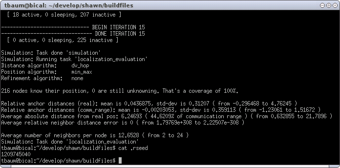
First, localization_evaluation prints the used algorithms (the ones we have written into the configuration file). Then, it prints some general information. 216 nodes computed successfully their position (remember that we set 9 nodes to be anchors, so 216 + 9 = 225 which is a coverage of 100%).

The next lines contain some additional information about the error rate of the computed positions. E.g., Average absolute distance from real pos is approximately 6 which is not a satisfactory result in a 100x100 world and a communication range of 14 (44.6209 percent as can be seen in the figure). In the end of the line, the minimal and maximal error are printed. The best positioned node is located 0.632855 units from its real position, whereas the worst one missed it by 21.7896 units.

The last line gives some information of the connectivity, and prints the average number of neighbors of the nodes (12.6528), as well as the minimum and maximum (2 and 24, respectively).

Seeing what happens

Figure XXX showed only textual statistics. On the one hand, very interesting and helpful for the one who evaluates such algorithms. But on the other hand it would be much more exciting if we can see the topology and the false positioned nodes. Therefore the localization application has an integrated visualization component. If invoked, the task localization_evaluation produces a postscript output of the topology. Change your configuration file as follows:

  random_seed action=load filename=.rseed
  ...
  localization_evaluation loc_ps_out=topology.ps

First, the random seed is reloaded to simulate the same scenario as before. Then, the task localization_evaluation becomes the parameter loc_ps_out that specifies the name of the postscript file that is used for output. After running

  ./shawn -f my_conf 

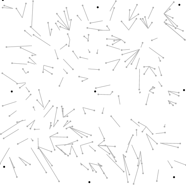
there is the file topology.ps in the current folder that contains the pages as shown in Figure XXX.

{| align="center" | | | |}

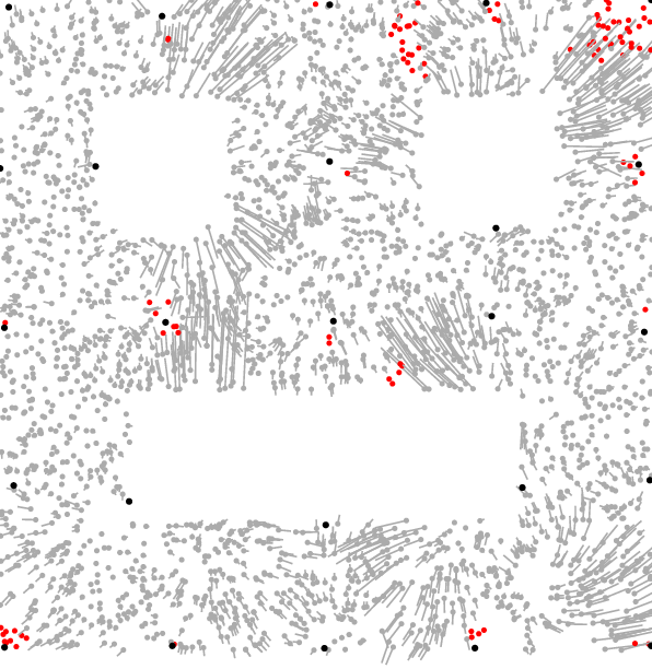
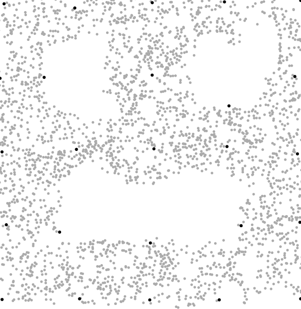
The black circles represent the anchors (nodes that know their real position), and the grey nodes represent ones that must compute their real position based on information distributed by the anchors . In the first image you can see additional lines from grey nodes to different positions. Here, the grey nodes are located at their real position, and the lines point to the position where the nodes think they are located. In the second image the nodes are on the positions where they think they are, whereas the third image shows the real topology.

The fact that many nodes point to the same location is based on both the chosen distance algorithm (DvHop) and positioning algorithm (MinMax). We will alter these parameters and compare the results next.

Comparing different Results

The previously used algorithms led to many nodes that computed the same position. In particular, this is based on the used distance algorithm that only uses hops (times of message forwarding) for distance estimation. But also the positioning algorithm MinMax tends to calculate similar positions from nearly similar data. Hence, let us change both algorithms as follows.

  loc_dist_algo=sum_dist
  loc_pos_algo=lateration

Now, the distance algorithm is based on estimation of the real distances. For now, the estimation is done with perfect_estimate that returns only correct values. But the next paragraph describes how to introduce ranging errors.

For positioning, Lateration is taken that generally computes more accurate values than MinMax. Look at the result of the simulation shown in Figure XXX.

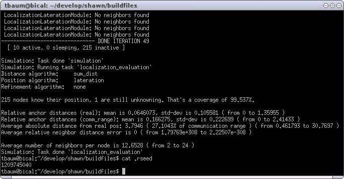
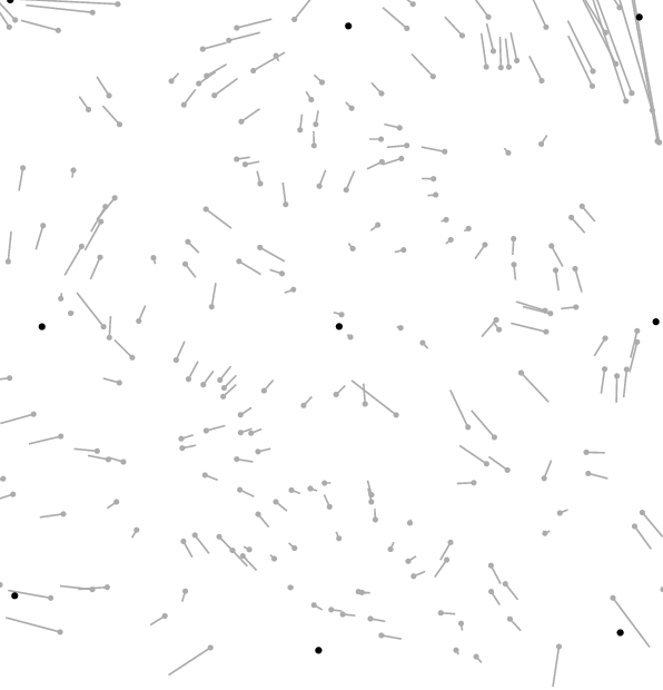
The most important difference is the average absolute distance from real position which dropped from 6.24693 to 3.7946 (or 44.6209% to 27.1043% in percent of communication range). Hence, a noticeable improvement. Figure XXX shows the result from the visualization.

{| align="center" | | | |}

As a result of using the alternative algorithms SumDist and Lateration, nodes are no longer positioned on equal positions. As already mentioned, this depends particularly on the different distance estimation. Instead of the previously used DvHop that computes distances from hops, SumDist measures each distance directly. So far, perfect distance estimation is used. That is, if a node measures the distance to another node, it obtains the correct value without any measurement errors. The introduction of such errors is described next.

Distance Estimation

When a node measures the distance to a neighbor, it can use the available Node Distance Estimate. There are three different types available. Perfect Estimate returns the real distance without any error. Absolute Error uses a uniform random variable for introducing errors, and Randomized Distance uses an arbitrary random variable. Because random variables are described later in more detail, the Absolute Error Distance Estimate is used first.

The task create_absolute_error_distance_estimate for adding such a distance estimate needs at least two parameters. The parameter name is used for unique identification, and error defines the span of the resulting deviation. There is also the optional parameter offset that can be used for a value that is added or subtracted on each estimation. Whenever a node requests a distance, the real distance plus the optional offset plus a random value in the range of [-\fraerror, +\fraerror] is returned. However, replace the line

  loc_est_dist=perfect_estimate 

with

  create_absolute_error_distance_estimate \
    name=abs_distest error=2.5
  loc_est_dist=abs_distest

Then, the resulting simulation looks as shown in Figure XXX.

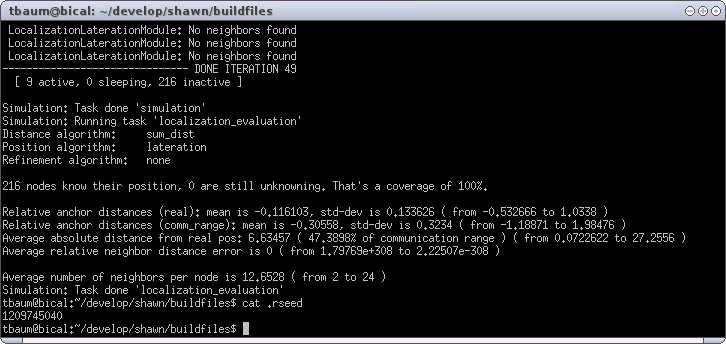
The average absolute distance error raised to 6.63457 (or 47.3898 in percent of communication range), and thus even exceeds the results from the first used DvHop. Note that the chosen error of 2.5 (-1.25..1.25) is an absolute value, and thus particularly influences nodes that are located close to each other. A relative Node Distance Estimates would be a wiser choice, but such objects are introduced later.

Topologies

In all previous examples the nodes were placed randomly in a rectangular plane. But Shawn does also allow for more complex topology generation. Therefore the application topology must be enabled (check via ccmake ../src from shawn/build_files that MODULE_APPS_TOPOLOGY is set to ON). The topology application provides different tasks for topology generation. One of them generates a network from XML files. As an example, create the file smiley.xml with the following content:

  <topology>
    <polygon blocking="0" type="outer">
      <vertex x="0" y="0"/>
      <vertex x="100" y="0"/>
      <vertex x="100" y="100"/>
      <vertex x="0" y="100"/>
    </polygon>
    <polygon blocking="1" type="hole">
      <vertex x="20" y="60"/>
      <vertex x="80" y="60"/>
      <vertex x="80" y="80"/>
      <vertex x="20" y="80"/>
    </polygon>
    <polygon blocking="1" type="hole">
      <vertex x="15" y="15"/>
      <vertex x="15" y="35"/>
      <vertex x="35" y="35"/>
      <vertex x="35" y="15"/>
    </polygon>
    <polygon blocking="1" type="hole">
      <vertex x="65" y="15"/>
      <vertex x="65" y="35"/>
      <vertex x="85" y="35"/>
      <vertex x="85" y="15"/>
    </polygon>
  </topology>

First, the file contains outer tags called topology that in turn contain at least one polygon. A polygon can be either an outer one or a hole. The former defines the area where nodes are placed. The latter can be used to define holes inside this area in which nodes are not allowed to be located.

When such a XML file has been created it must be loaded by the application. This is done by the simulation task xml_polygon_topology which gets the parameters name for identifying the polygon by an unique name, and file that contains the filename of the XML file (here, it would be smiley.xml).

After the polygon has been loaded, nodes must be created in the given area. Therefore the simulation task populate must be called. It expects the parameters topology (for example, the above generated polygon that is identified by the given name), a point generator by point_gen, and the amount and type of processors.

Create the following configuration file:

  random_seed action=load filename=.rseed

  prepare_world edge_model=list comm_model=disk_graph \
    transm_model=stats_chain \
    range=4

  chain_transm_model name=reliable

  loc_est_dist=perfect_estimate
  loc_dist_algo=sum_dist
  loc_pos_algo=lateration
  loc_ref_algo=none

  xml_polygon_topology name=xml_top file=smiley.xml
  populate topology=xml_top point_gen=uniform_2d count=3000 \
    processors=localization

  localization_anchor_placement anchor_placement=outer_grid \
    placed_anchor_cnt=25

  simulation max_iterations=20

  localization_evaluation loc_ps_out=topology.ps

Running this configuration in Shawn results in Figure XXX.

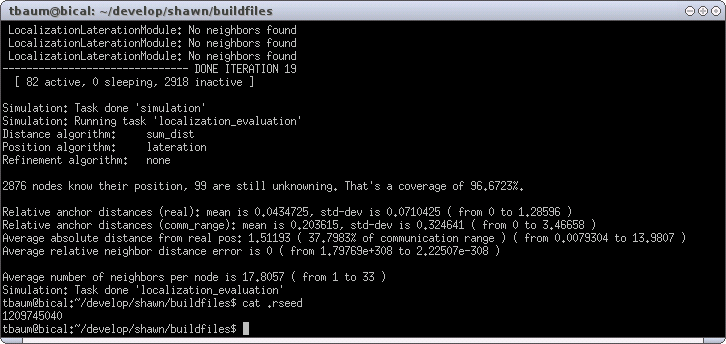
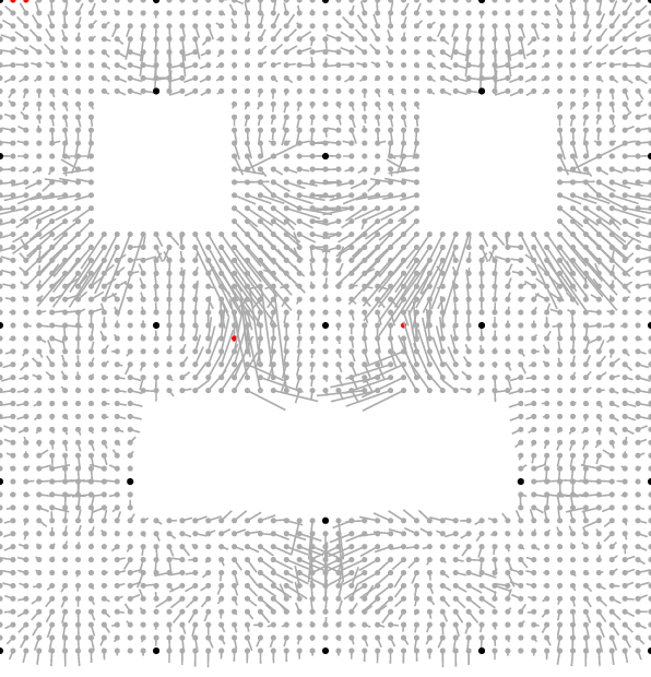
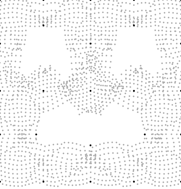
The corresponding visualization is shown in Figure XXX.

{| align="center" | | | |}

The nodes have been populated randomly in the specified area, because uniform_2d point generation was chosen. There are also other alternatives for point generation. For example, replace the populate-task in the configuration file with the following line.

  populate topology=xml_top point_gen=lattice spacing=2 \
	   count=3000 processors=localization

The result is visualized in Figure XXX.

{| align="center" | | | |}