-
Notifications
You must be signed in to change notification settings - Fork 170
De noising Filters
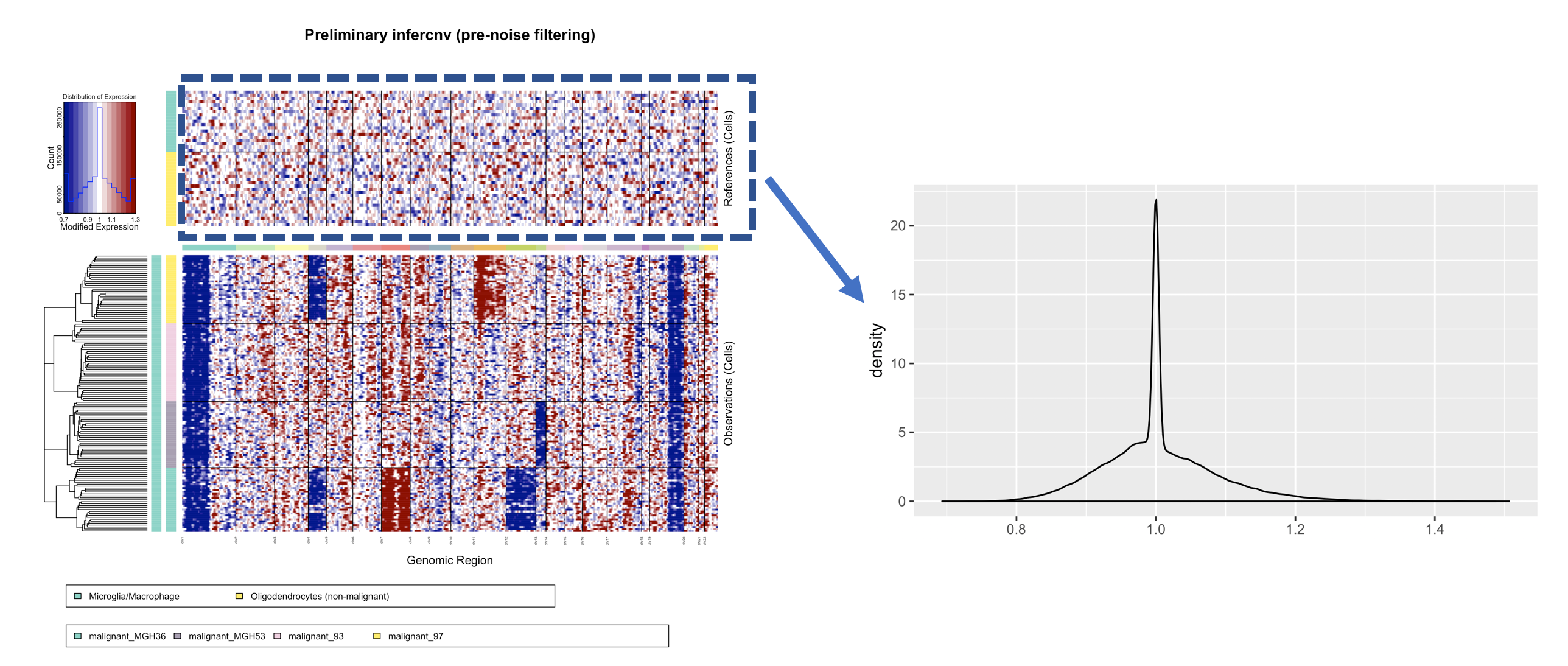
These de-noising filter options are available for manipulating the residual expression intensities with the goal of reducing the noise (residual signal in the normal cells) while retaining the signal in tumor cells that could be interpreted as supporting CNV.
The residual normal signal is derived from the preliminary inferCNV object, which has been smoothed, centered, and the mean of the normal (reference) cells subtracted:

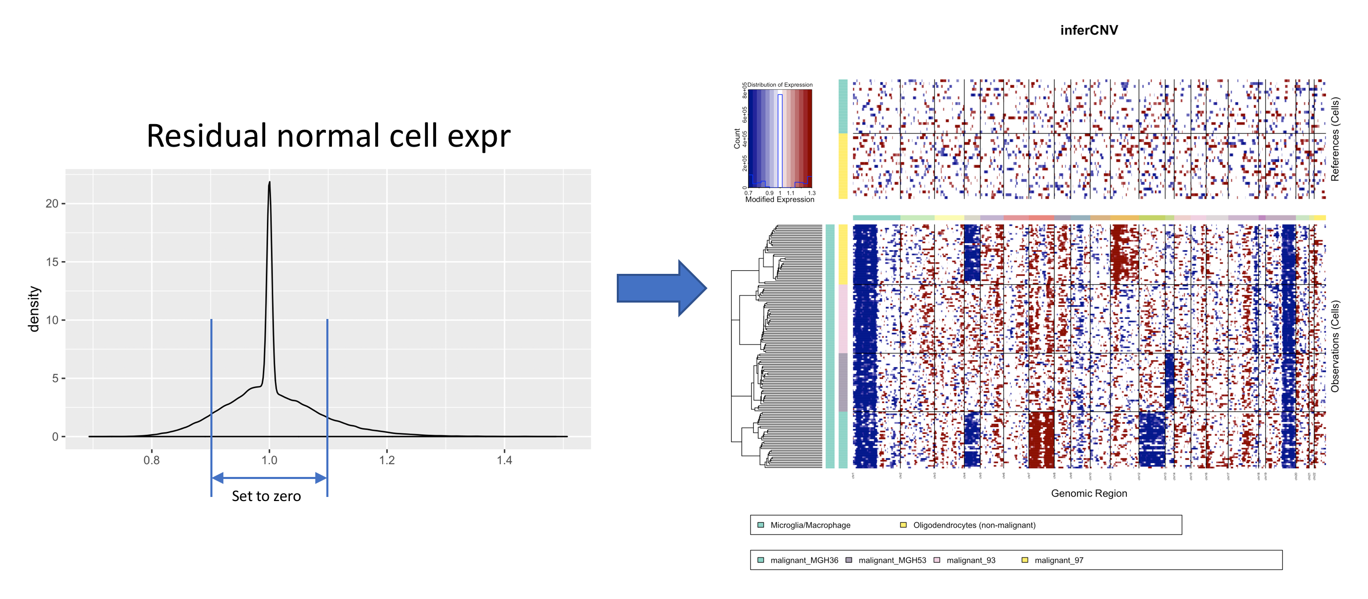
A specific threshold deviation from the mean can be set using the 'noise_filter' attribute, as shown below:
infercnv_obj = infercnv::run(infercnv_obj,
                             cutoff=1, # cutoff=1 works well for Smart-seq2, and cutoff=0.1 works well for 10x Genomics
                             out_dir=out_dir,
                             cluster_by_groups=T,
                             plot_steps=F,
                             denoise=T,
                             noise_filter=0.1   ## hard thresholds
                             )

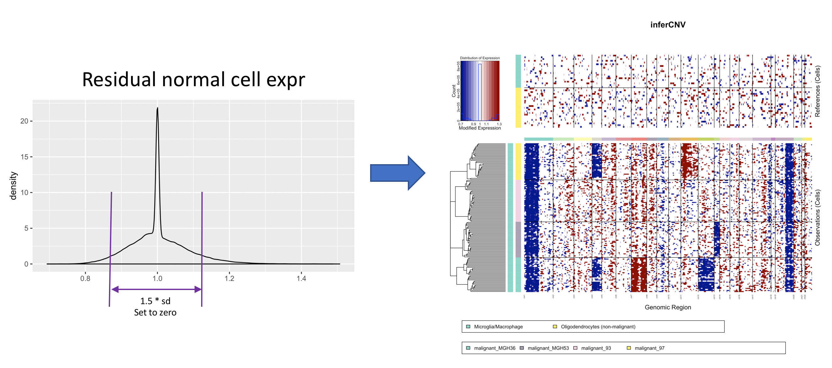
By default, the hard cutoffs for denoising are computed based on the standard deviation of the residual normal expression values. This thresholding can be adjusted using the 'sd_amplifier' setting. For example, we can use 1.5 * the standard deviation for filtering like so:
infercnv_obj = infercnv::run(infercnv_obj,
                             cutoff=1, # cutoff=1 works well for Smart-seq2, and cutoff=0.1 works well for 10x Genomics
                             out_dir=out_dir,
                             cluster_by_groups=T,
                             plot_steps=F,
                             denoise=T,
                             sd_amplifier=1.5  ## set dynamic thresholding based on the standard deviation value.
                             )
Instead of applying a strict threshold, you can apply a filtering gradient by applying a sigmoidal function that reduces intensities near the mean more than intensities more distant from the mean. An example of applying this 'noise_logistic' is shown below.
infercnv_obj = infercnv::run(infercnv_obj,
                             cutoff=1, # cutoff=1 works well for Smart-seq2, and cutoff=0.1 works well for 10x Genomics
                             out_dir=out_dir,
                             cluster_by_groups=T,
                             plot_steps=F,
                             denoise=T,
                             sd_amplifier=3,  # sets midpoint for logistic
                             noise_logistic=TRUE # turns gradient filtering on
                             )
The midpoint for the sigmoidal curve (logistic function) is set based on the sd_amplifier (or alternative, fixed value at a 'noise_filter' setting), and this is enabled by setting 'noise_logistic=TRUE'.
For any of the types of denoising (even disabled) explained above, an add-on median filtering can be applied to smooth the visual output of inferCNV. To do so, you simply need to apply the median filtering method on the inferCNV object and plot it again.
infercnv_obj_medianfiltered = infercnv::apply_median_filtering(infercnv_obj)

infercnv::plot_cnv(infercnv_obj_medianfiltered,
                   out_dir='../example_output/',
                   output_filename='infercnv.median_filtered',
                   x.range="auto",
                   x.center=1,
                   title = "infercnv",
                   color_safe_pal = FALSE)
The filtering takes into account chromosomes and the clusters or subclusters that have been defined as boundaries. It also keeps the hierarchical clustering previously defined intact in order for it to be representative of how it was obtained.
Using the inferCNV object obtained running the denoising via sigmoidal (see above), the resulting figure can be seen below.

- InferCNV Home
- Quick Start
- Installing inferCNV
- Running InferCNV
- Applying Noise Filters
- Predicting CNV via HMM
- Bayesian Mixture Model
- Tumor heterogeneity - define tumor subclusters
- Interpreting the Figure
- Inputs to InferCNV
- Outputs from InferCNV
- More inferCNV example data sets
- Using 10x data
- Interactively navigating data using the Next Generation Heatmap Viewer
- Extracting HMM features
- FAQ and common issues