-
Notifications
You must be signed in to change notification settings - Fork 3
Samples
In the following, we demonstrate how to use irbasis database. The irbasis database is available in Python and C++. irbasis can calculate the IR basis functions, its Fourier transform, the derivatives and corresponding singular values.
In the following, we assume that you have installed the irbasis Python library via pip. If not, please modify the sample script files appropriately to specify the location of a database file (see a comment in api.py).
Some of sample Python scripts depend on scipy and matplotlib.
- Usage of interface (Python, C++)
- Plotting the IR basis function (Python)
- Step by step examples (Python)
- Transformation between representations (Python)
- Sparse sampling
- How to use from Julia
You can download api.py and save it to your working directory. Then, please run the following command
python api.pyYou can study also our step-by-step examples in a jupyter notebook.
You can download api.cpp and step_by_step_examples.cpp to your working directory. After copying irbasis.hpp into the same directory, you can build the sample program as follows (see compile.sh).
g++ api.cpp -o api -I /usr/local/include -L /usr/local/lib -lhdf5 -DNDEBUG -O3
g++ step_by_step_examples.cpp -o step_by_step_examples -I /usr/local/include -L /usr/local/lib -lhdf5 -DNDEBUG -O3
Here, we assume that the header file and the library file of the HDF5 C library are installed into "/usr/local/include" and "/usr/local/lib", respectively. When running the executable, irbasis.h5 must exist in your working directory.
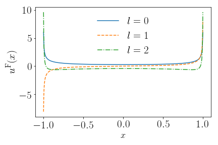
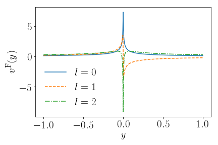
This sample code uv.py plots the IR basis functions u(x) and v(y) for Lambda = 1000 and fermions.


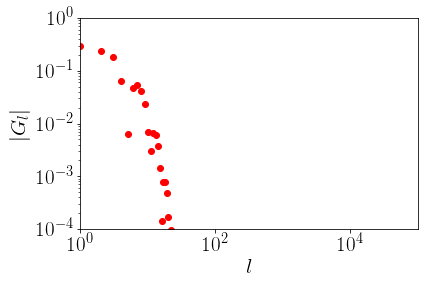
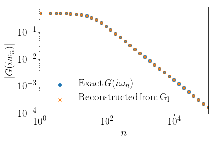
In this sample, we demonstrate how to compute expansion coefficients of a given imaginary-time Green's function G_l and transform an imaginary-time Green function to one with the Matsubara frequency i\omega_n. We choose the insulator-like spectrum with the pole at \omega = 2 as the model. The technical details are given in Appendix B of N. Chikano et al. arXiv:*****. The parameters are beta = 100, Lambda = 1000 with fermions.
You can simply download giwn.py and save it to your directory. Then, type
python giwn.py This python file generates two figures as shown below. The upper figure plots the absolute value of expansion coefficients G_l with respect to l. The lower plots the exact G(i\omega_n) and G(i\omega_n) converted from G_l. The former is calculated by G(i\omega_n) = 1/(i\omega_n - pole).


Here is a jupyter notebook which demonstrates the sparse sampling techniques proposed in arXiv:1908.07575.
irbasis can be used from Julia through PyCall.jl. Here is a jupyter notebook.