A #SmartCityHack project rolled by Alex, Daniel, Steven, and Zack!
Abstract: using a live feed provided by the City of Auburn, we can programmatically determine if Auburn Tigers fans have begun rolling Toomer's Corner by analyzing images via Canny edge detection and analysis of gradient vectors. These techniques rely on very particular geometric properties of the phenomenon we are trying to detect. This repository instead seeks to accomplish the same via a more general image analysis algorithm, often termed Principal Component Analysis, in order to generalize the image-detection engine to various other real-world applications.
Our live implementation of Is Toomer's Corner Being Rolled Right Now relies on Canny edge detection to preprocess images and then analyses the gradient vectors in the Canny-ized image in order to guess at whether Toomer's Corner is covered in celebratory toilet paper.

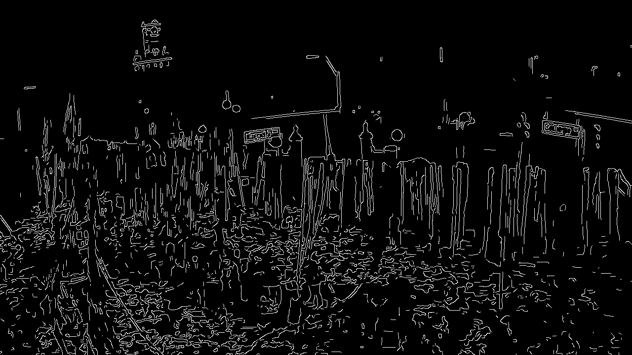
The Canny-gradient algorithm reliably detects large numbers of near-vertical and vertical lines in an image, and thus provides a good guess at whether celebration is happening on the corner. However, the limits of such an algorithm are apparent as soon as one seeks to generalize to the detection of other phenomenon--it is not clear that the geometric properties of a usual image will be significantly different from those of a unusual image. In essence, we lucked out, simply because of gravity, and Canny-gradient detection takes advantage of that position.
It became clear to us that if we wanted an image-detection algorithm that was actually anything like useful, we'd need something more general. Also, we cannot anticipate the geometric properties that will distinguish unusual images from usual images.
Our solution: we will train our algorithm to spot those differences through statistical analysis of a large set of usual images.
Using these methods, we hope to be able to detect arbitrary unusual images, which may then be flagged for analysis by a secondary image processor or for human intervention/action.
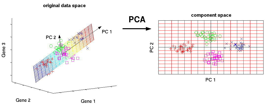
We use computationally-expensive Principal Component Analysis (abbreviated PCA) to analyze training data representative of presumably usual images. We may then use computationally-cheap image analysis methods to compare a live image to the results from the training data, and determine whether the live image is usual or unusual.
We ran our trained image analyzer on archival images of Toomer's corner under various amounts of toilet paper, as well as on several silly images.
In order to ballpark a baseline score, we first ran the image analyzer on 20 unrolled images. The images and their scores can be found in our sample-data repository, but here are the scores for the convenience of the reader:
 pca-unrolled-from-archive.txt
 -----------------------------
 img: 2015-02-21_11-28-42.jpg    score: 1942.333056456192
 img: 2015-02-21_11-28-43.jpg    score: 1461.0635427474256
 img: 2015-02-21_11-28-44.jpg    score: 1212.8302947918517
 img: 2015-02-21_11-28-45.jpg    score: 1237.291162568768
 img: 2015-02-21_11-28-46.jpg    score: 929.3443587938181
 img: 2015-02-21_11-28-47.jpg    score: 1033.5302920375207
 img: 2015-02-21_11-28-48.jpg    score: 910.4956889919005
 img: 2015-02-21_11-28-49.jpg    score: 1214.7154974935213
 img: 2015-02-21_11-28-50.jpg    score: 1241.1939105821282
 img: 2015-02-21_11-28-51.jpg    score: 1556.7247118298226
 img: 2015-02-21_11-28-52.jpg    score: 1955.210662398523
 img: 2015-02-21_11-28-53.jpg    score: 1990.1815251259202
 img: 2015-02-21_14-03-33.jpg    score: 633.9996327567347
 img: 2015-02-21_14-03-34.jpg    score: 612.1522207034938
 img: 2015-02-21_14-03-35.jpg    score: 547.5671276398446
 img: 2015-02-21_14-03-37.jpg    score: 517.4147807336952
 img: 2015-02-21_14-03-38.jpg    score: 532.8497394798661
 img: 2015-02-21_14-03-40.jpg    score: 579.2520644414814
 img: 2015-02-21_14-03-41.jpg    score: 475.75492042371064
 img: 2015-02-21_14-03-42.jpg    score: 466.4007149599398
Recall that a higher score indicates (presumably) a more unusual image. The scores range from 466 to 1990. The average score is 1052, with a standard deviation of 520.

Lowest-scoring unrolled image, at 466.

Average-scoring unrolled image, at 1052.

Highest-scoring unrolled image, at 1990.
Next we applied the trained image analyzer to archival images of the corner in a rolled state.
 pca-rolled-from-archive.txt
 ---------------------------
 img: 2015-02-21_11-05-28.jpg    score: 1114.937424911573
 img: 2015-02-21_11-05-29.jpg    score: 1883.2568935238596
 img: 2015-02-21_11-05-30.jpg    score: 2565.4953370713756
 img: 2015-02-21_11-05-31.jpg    score: 3149.014080638789
 img: 2015-02-21_11-05-32.jpg    score: 3176.393056241723
 img: 2015-02-21_11-05-33.jpg    score: 2729.9825766400454
 img: 2015-02-21_11-05-34.jpg    score: 3217.4583899413115
 img: 2015-02-21_11-05-35.jpg    score: 2717.291894576775
 img: 2015-02-21_11-05-36.jpg    score: 3220.3516950300573
 img: 2015-02-21_11-05-37.jpg    score: 3104.428909807628
 img: 2015-02-21_11-05-38.jpg    score: 3008.448707765287
 img: 2015-02-21_11-05-39.jpg    score: 2930.590774095586
 img: 2015-02-21_11-05-40.jpg    score: 3074.7927182318617
 img: 2015-02-21_11-05-41.jpg    score: 3142.80122502018
 img: 2015-02-21_11-05-42.jpg    score: 2633.399959459505
 img: 2015-02-21_11-05-43.jpg    score: 1886.859147965476
 img: 2015-02-21_11-05-44.jpg    score: 1652.3006235699575
 img: 2015-02-21_11-05-45.jpg    score: 1695.3782454751806
 img: 2015-02-21_11-05-46.jpg    score: 1277.046866929809
 img: 2015-02-21_11-05-47.jpg    score: 1257.333667962419
 img: 2015-02-21_11-27-02.jpg    score: 1888.5827181736904
 img: 2015-02-21_11-27-03.jpg    score: 1811.4594379933799
 img: 2015-02-21_11-27-04.jpg    score: 1444.3221269226963
 img: 2015-02-21_11-27-05.jpg    score: 1618.7795752141603
 img: 2015-02-21_11-27-06.jpg    score: 2012.79366290431
 img: 2015-02-21_11-27-07.jpg    score: 1976.7977733376913
 img: 2015-02-21_11-27-08.jpg    score: 2052.8985671872374
 img: 2015-02-21_11-27-09.jpg    score: 2765.798453929485
 img: 2015-02-21_11-27-10.jpg    score: 2259.6502811705973
 img: 2015-02-21_11-27-11.jpg    score: 2446.266801980547
 img: 2015-02-21_11-27-12.jpg    score: 2752.0940631728427
 img: 2015-02-21_11-27-13.jpg    score: 2582.8439573245505
 img: 2015-02-21_11-27-14.jpg    score: 2016.8654166552508
 img: 2015-02-21_11-27-15.jpg    score: 1847.0678359339888
 img: 2015-02-21_11-27-16.jpg    score: 1262.4819653042787
 img: 2015-02-21_11-27-17.jpg    score: 1324.0551850898114
 img: 2015-02-21_11-28-33.jpg    score: 1051.7191761887595
 img: 2015-02-21_11-28-34.jpg    score: 1797.009819497115
 img: 2015-02-21_11-28-35.jpg    score: 1813.9605223921967
 img: 2015-02-21_11-28-36.jpg    score: 3039.579335248384
 img: 2015-02-21_11-28-37.jpg    score: 2713.2471702500943
 img: 2015-02-21_11-28-38.jpg    score: 2118.547098323372
 img: 2015-02-21_11-28-39.jpg    score: 1784.952348517634
 img: 2015-02-21_11-28-40.jpg    score: 1344.291369478608
 img: 2015-02-21_11-28-41.jpg    score: 1397.4266536226673
 img: 2015-02-21_11-28-54.jpg    score: 1375.4927016186023
 img: 2015-02-21_11-28-55.jpg    score: 1859.5455368023918
 img: 2015-02-21_11-28-56.jpg    score: 2129.247432745011
 img: 2015-02-21_11-28-57.jpg    score: 2077.3774710946036
 img: 2015-02-21_11-28-58.jpg    score: 2278.4474327405037
 img: 2015-02-21_11-28-59.jpg    score: 2735.869280054003
 img: 2015-02-21_11-29-00.jpg    score: 1361.9771306435246
The scores for rolled images range from 1051 to 3220, with average score 2161 and standard deviation of 655.

Lowest-scoring rolled image, at 1051.

Average-scoring rolled image, at 2161.

Highest-scoring rolled image, at 3220.
Next we tested the generality of our image analyzer by scoring several highly unusual images representative of road closure due to dinosaur attack.

Dinosaur Comics' T-Rex and Toy Story's Rex scored a very respectable 2837, not too shabby!

The police barricade scored a whopping 5219.
The week leading up to the competition deadline, we began scraping the Toomer's live web cam feed for periodic frames.
We managed to collect roughly 10000 still frames, stored as 1280 x 720 32-bit color .png files.
PCA relies on performing singular value decomposition (abbreviated SVD) of the matrixized version of our training data (the so-called principal components are those singular vectors corresponding to an arbitrary but fixed number of the largest singular values). We first represent each image as a high-dimensional row vector (2,746,800 dimensions, one dimension for each x-coordinate, y-coordinate, and color channell of each pixel). We form the 2,746,800 by 10,000 matrix whose rows are the vectorized training images, and we perform the SVD in order to find the singular vectors. These singular vectors, when translated by the average of our training images, span the best-fit hyperplane to our training images. We may then measure the unusualuality of an image by calculating it's euclidean distance to the best-fit hyperplane.
We quickly determined that this method, as described, was inadequate, particularly when the kernel complained about not having 6TB of RAM to allocate and terminated our training program before completion.
Our solution was twofold:
-
We decided to chop each 1280x720 image into 144 smaller 80 by 80 sectors, train each sector separately, and then analyze live images on a sector-by-sector basis, aggregating the scores via square sum into one composite score.
-
We still found it necessary to reduce the resolution from 80 by 80 to 20 by 20, losing information in the process but allowing us to proceed.
Now, instead of performing one SVD on a single 2,746,800 by 10,000 matrix, we perform SVD on 144 separate 1,000 by 10,000 matrices, finding the best-fit hyperplane for each of the 144 sectors.
Training our image processor is computationally expensive and requires ample data representing usual images. Once our processor is trained, however, we use the results of the training to quickly score live images, where higher scores mean the image is more unusual.
-
Training images are cut into 144 smaller 80 by 80 sectors and stored to disk by
preconvert.hsviapreconvert.sh. -
SVD is applied in each sector, generating the best-fit hyperplane, which is saved as a text file in the same directory, by
train.hsviatrain.sh. -
Some sectors might be more variable than other sectors (eg, sky sectors vs road sectors). To correct for this possibility, we apply the image processor to the training data, to measure the tendency for the training data to fall outside of the best-fit hyperplane. This step is handled by
genstats.hsviagenstat.sh, and the average distance for each sector is stored inavgdist.txtin the corresponding directory. At this stage, training is complete. -
extract.shcopies the training data into a format that the deployment image processor expects.
The entire training process took about 8 hours of computation on my AMD-64 machine running Ubuntu 14.04 with 8 GB of RAM.
The deployment image processor reads the training data (we ended up having about 211 MB) and calculated the square-sum aggregate score of the distances of each sector to that sectors hyperplane.
Scoring an individual image takes between 1.5 and 3 minutes per image on my machine. Much of this is filesystem overhead associated to reading the training data, and in a refined implementation would be eliminated by holding the training data in RAM continually.
Our results indicate to us that Principle Component Analysis can be used as a second-generation image-analysis engine for IsToomersCornerBeingRolledRightNow.com that can be generalized to a wide variety of other urban applications, including early warning systems and real-time traffic/transit information and management.
Our humble proof-of-concept was limited by our relatively small amount of training data (ideally we would want to accumulate training data over the course of several months) and the physical limitation of our desktop computers. We believe that with more sophisticated hardware and with a bit of code tweaking to optimize for disk reads and garbage collection, we will have a highly-general image analysis algorithm, capable of detecting arbitrary unusual activity in virtually any setting.
Haskell source code. Compiles to a library.
This library contains utility functions for loading, converting, and manipulating images.
Haskell source code. Compiles to library.
This library contains the functions needed to perform principal component analysis on vectorized data.
Haskell source code. Compiles to an executable.
We're passed (1) the path to a directory that contains training data
and (2) the path to an image from the camera feed.
Chops up the image into 144 smaller 80 by 80 sectors, and calculates, for
each sector, the distance to
the linear-regression hyperplane for that sector, and divides by the
training data's average distance to the same hyperplane.
Returns, to stdout, the square sum of the scores described above.
Higher number means the image is more unusual.
BASH script.
We're passed (1) a directory that contains sample data and the results of the training process and (2) the directory in which we want to save only the results. This script will extract the results of training and place them in a separate directory, preserving subdirectory structure.
Haskell source code. Compiles to executable.
We're passed a directory path .../chopped/someNumber containing
training data (presumably 'typical' images from the camera feed) and
the hyperplane.txt generated by train.hs.
We compare each image to the hyperplane, take the mean distance,
and save that in a text file, called avgdist.txt, in the same directory.
This completes analysis of the training data.
BASH script wrapper for genstats.hs
We're passed the path of the directory containing chopped images and
hyperplanes. This script runs genstats on each of the 144 subdirectories,
so that each directory should end up containing avgdist.txt.
Haskell source code. Compiles to executable.
We're passed the path to an image. We expect that image to be 1280 by
720, and we chop that image into 144 smaller 80 by 80 pieces, saving the
pieces with the same file name as the original but in numbered
subdirectories, chopped/1, chopped/2, etc.
BASH script wrapper for preconvert.hs
We're passed a directory that contains thousands of images. This
script runs preconvert on each image. Results should be 144 subdirectories
chopped/1, chopped/2, etc., each of which should contains thousands of tiny images.
Haskell source code. Compiles to executable.
We're passed (1) the path to a directory and (2) an integer. Saves a hyperplane (dim = 2nd arg) that is the linear regression of all of the images in the directory to hyperplane.txt in the same directory.
BASH script wrapper for train.hs
We're passed the path to a directory containing chopped images. This script runs train on each subdirectory, which analyzes the images contained inside and writes a file, hyperplane.txt, into that subdirectory.