DeepRibo

Introduction

DeepRibo is a deep neural network created by Clauwaert. J et. al. for the annotation of Open Reading Frames (ORF) in prokaryotes using ribosome profiling signal and binding site patterns (Shine-Dalgarno region). The package is written in python 3 and uses the PyTorch library for deep learning purposes. A model has been trained and evaluated using seven ribo-seq datasets. More information is available in the published article:

DeepRibo: A deep neural network for the precise gene annotation of prokaryotes by combining ribosome profiling signal and binding site patterns

Jim Clauwaert, Gerben Menschaert, Willem Waegeman

Nucleic Acids Research 2019

The pre-trained model, present in the directory models, can be applied to annotate any prokaryotic genome for which ribosome profiling data is available. The use of this model is the recommended procedure when applying DeepRibo for personal use. Although the models are trained making use of GPU technology, annotations made by DeepRibo should take no more than two hours of processing time in case computations are done by CPU's (~10 minutes on GPU). In addition, several scripts are present which make it possible to train new models using custom data and model architecture. It is strongly recommended to use GPU infrastructure for the training of new models using DeepRibo.

Methodology

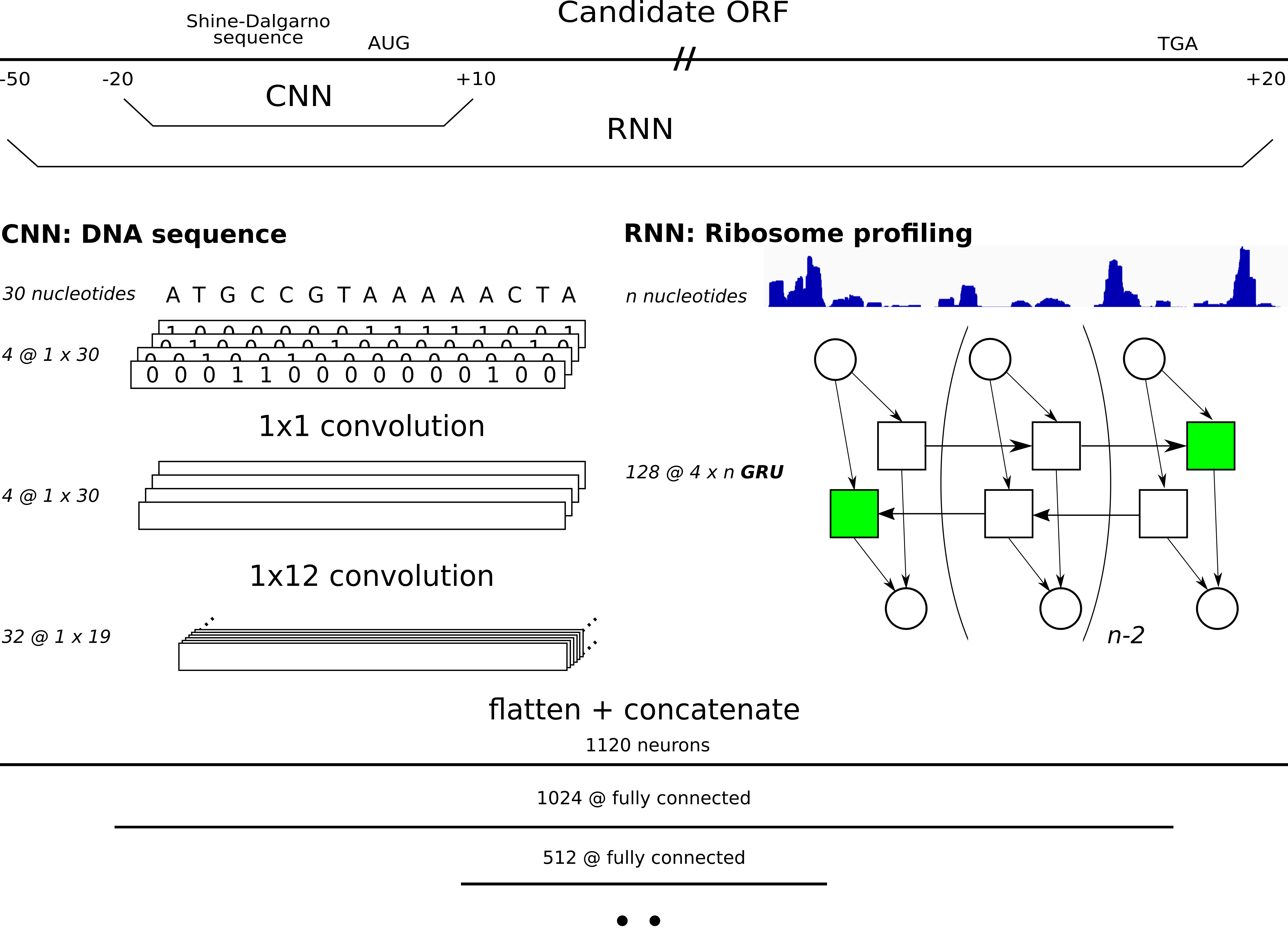
DeepRibo is a deep neural network applying both architectures from convolutional neural networks for motif detection and recurrent neural networks to process ribosome profiling signal. The model evaluates all possible ORFs (given a set of start and stop codons) with mapped reads (ribosome profiling) in the genome, assigning probabilities to processed candidate ORFs. A more in depth explanation about the training procedure and results are given in the release article.

Installation

To use DeepRibo, simply clone the repository in your working directory and install the necessary python libraries:

git clone https://github.com/Biobix/DeepRibo.git

DeepRibo uses following packages for Python 3.8:

	numpy
	pandas
	scikit-learn
	biopython
	pytorch

Install PyTorch at www.pytorch.org. Make sure the software installed supports the available hardware. In case PyTorch loses backwards compatibility, this package has been created using PyTorch v0.4 and has been successfully tested up to PyTorch 1.4.

Pretrained models

For usage, we recommend using the model trained on the combination of seven ribosome profiling datasets. This model is featured as models/DeepRibo_model_v1.pt

All seven models discussed in the Full Article are located in models/article/, and can be directly used to annotate TIS/ORF using personal data. DeepRibo has been evaluated using seven different ribosome profiling experiments. To ensure overall performance, seven models were trained each time excluding one of the seven datasets for testing. These pretrained models are named by the dataset excluded from training, and therefore also the dataset from which the performance measures are obtained. User data has to be first parsed using DataParser.py. Before any predictions can be made, candidate ORFs with low signal are filtered out. To determine the cut-off values on the user data the R-script src/s_curve_cutoff_estimation.R is used. In case no annotation data is available (de novo), a conservative value of 0.12 and 0.27 can be taken for the coverage and RPKM cutoff, respectively. Finally, predictions are made by running DeepRibo.py predict.

User Guide

src/DataParser.py and src/DeepRibo.py are the main scripts from which all functionalities can be accessed. More information about these functions can be obtained using the -h flag.

Data Preparation

First, data has to be converted into the required format. DataParser.py takes care of this with minimal effort. Several files are required to successfully parse the data. In short, the ribosome profiling data of elongating ribosomes has to be compiled into four bedgraph files. These contain the coverage signals of all reads and the mapped A/P profiles (reads mapped to one site). The following steps are performed:

• read adapters are trimmed
• rRNA sequences are filtered out and only uniquely mapped reads are used
• a 12nt offset from the 3' end of the read is used to map reads to a single position on the genome.

Transforming mapped reads from a .bam format to a .bedgraph format can be achieved using bedtools genomecov

Parsing Data

python DataParser.py -h

positional arguments:
  sense_cov             Path to bedgraph containing sense riboseq data
			(elongating coverage)
  asense_cov            Path to bedgraph containing antisense riboseq data
			(elongating coverage)
  sense_elo             Path to bedgraph containing sense riboseq data
			(elongating A-site)
  asense_elo            Path to bedgraph containing antisense riboseq data
			(elongating A-site)
  fasta                 Path to fasta containing genome sequence
  destination           Path to output destination. This path must contain two
			folders named 0 and 1

optional arguments:
  -h, --help            show this help message and exit
  -g GTF, --gtf GTF     Path to gtf/gff containing annotation (default: None)
  -s START_TRIPS [START_TRIPS ...], --start_trips START_TRIPS [START_TRIPS ...]
			list of tripletsconsidered as possible start codons
			(default: ['ATG', 'GTG', 'TTG'])
  -p STOP_TRIPS [STOP_TRIPS ...], --stop_trips STOP_TRIPS [STOP_TRIPS ...]
			list of tripletsconsidered as possible stop codons
			(default: ['TAA', 'TGA', 'TAG'])

DeepRibo makes predictions on all candidate ORFs present within a genome. Therefore, samples are generated by iterating over the genome an selecting regions delimited by any of the codons given by --start_trips and --stop_trips. When parsing a dataset for training purposes, an assembly file is necessary to create a set of positive samples (CDS entries). No assembly file is required for datasets on which predictions are made. However, the S-curve methodology uses the positive labels for the estimation of the cut-off values. In case no assembly file is available, a conservative cut-off value can be chosen by evaluating other datasets. As the exclusion of data is mainly important for training, small variations on these cut-off values should not pose any major discrepancies between the predictions.

When running Dataparser.py, two filetypes for each ORF present in te genome are created. *_seq.pt is the pickled binary image of the 30 nucleotide region covering the Shine-Dalgarno region ([-20,10]). *_reads.pt contains a vector with the riboseq coverage signal for each ORF. For each ORF present in the gff/gtf file (feature column annotated as CDS) a positive label is attributed. All samples will accordingly be be listed under <dest>/0 (negative label) or <dest>/1 (positive label).<dest>/data_list.csv contains a list of all samples with metadata. This file will be read and processed by the custom data loader used by DeepRibo.py. The parsed data of multiple datasets should all be present in one folder, according to the following structure:

DATA
├── ecoli (destination)
│   ├── 0
│   │   ├ ...
│   ├── 1
│   │   ├ ...
│   ├── data_list.csv
├── bacillus (destination)
│   ├── 0
│   │   ├ ...
│   ├── 1
│   │   ├ ...
│   ├── data_list.csv
├── ...

Training a model

This step is only necessary to train a custom model. For default usage of DeepRibo, predictions are used using one of the pretrained models.

After all data has been processed, a model can be trained. Any combination of datasets present in the DATA folder can be used for training/testing.

python DeepRibo.py train -h

Train a model

positional arguments:
  data_path             path containing the data folders for training and
			testing

optional arguments:
  -h, --help            show this help message and exit
  --train_data TRAIN_DATA [TRAIN_DATA ...]
			train data folder names present in the data path
			(default: [])
  --valid_size VALID_SIZE
			percentage of train used as validdata (default: 0.05)
  -r RPKM [RPKM ...], --rpkm RPKM [RPKM ...]
			minimum cutoff of RPKM values to filter the training
			data (default: None)
  -c COVERAGE [COVERAGE ...], --coverage COVERAGE [COVERAGE ...]
			minimum cutoff ofcoverage values to filter the
			training data, these are given in the same order.
			(default: None)
  -d DEST, --dest DEST  path to which the model is saved (default: pred)
  -b BATCH_SIZE, --batch_size BATCH_SIZE
			training batch size (default: 256)
  -e EPOCHS, --epochs EPOCHS
			training epochs (default: 20)
  -g GRU_NODES, --GRU_nodes GRU_NODES
			size of the hidden state of the GRU unit (default:
			128)
  -l {1,2}, --GRU_layers {1,2}
			amount of sequential GRU layers (default: 2)
  -B [GRU_BIDIRECT], --GRU_bidirect [GRU_BIDIRECT]
			use of bidirectional GRU units (default: True)
  -m COV_MOTIFS, --COV_motifs COV_MOTIFS
			amount of motifs (conv kernels) used by the
			convolutional layer (default: 32)
  -n FC_NODES [FC_NODES ...], --FC_nodes FC_NODES [FC_NODES ...]
			nodes per layer present in the fully connected layers
			of DeepRibo (default: [1024, 512])
  --model_type {CNNRNN,CNN,RNN}
			Use CNNRNN, CNN or RNN architecture (default: CNNRNN)
  --num_workers NUM_WORKERS
			numbers of CPU units used for dataloading (default: 0)
  --GPU                 use of GPU (RECOMMENDED) (default: False)
  -v, --verbose         more detailed progress bar (default: False)

During training, the model's weights are saved after each epoch in the destination folder -d. A json object is furthermore created containing all of the performance metrics for the training/testing data. These performance metrics include the cross-entropy loss, acceracy, Area Under the Roc Curve (AUC-ROC) and Area under the Precision-Recall Curve (PR-AUC). All of the model's parameters are furthermore saved in this file. When training the model, cut-off values for both the training data and test data, based upon the minimal coverage and RPKM values of each sample, are given to filter out data with low to non-existent signal (see Article). two cut-off values have to be given for each dataset used for training/testing (r and c), and are required to be in the same order as the dataset names given by --train_data. To obtain the right values for each dataset, an R script is provided. Make sure to install the SiZer package before use. The function get_cutoff_values is listed in src/s_curve_cutoff_estimation.R. Simply run the script with the required parameters to obtain these values after parsing the data. This function will not work with the mock data provided on this GitHub repository.

# start R	
R
# load the functions from the script
>source('s_curve_cutoff_estimation.R')
# list the dataset and the path to which the png figure is stored
>get_cutoff_values(path="../data/processed/<your data>/data_list.csv", dest="figure")
$min_RPKM
  ....
$min_coverage
   	  ....

Custom architectures of DeepRibo can be trained using a variety of parameters available when running DeepRibo.py. Specifically, --GRU_nodes, --GRU_layers, --GRU_bidirect, --COV_motifs and --FC_nodes can be used to set the hidden nodes of the GRU memory cell, the amount of layers, whether to use a bidirectional GRU, the amount of kernels used by the convolutional layer, and the amount of layers and nodes used in the fully connected layers of DeepRibo. The model type can be set using --model_type, making it possible to train a model using only the CNN or RNN partition of DeepRibo. Default values constitute the hyperparameters used to build the provided models.

Making predictions

Once a model has been trained it can be used to make predictions on any other data you have parsed. For more information about the required parameters simply use the help flag:

python DeepRibo.py predict -h

Create predictions using a trained model

positional arguments:
  data_path             path containing the data folders for predictions

optional arguments:
  -h, --help            show this help message and exit
  --pred_data PRED_DATA
			data folder name present in the data path used to make
			predictions on (default: None)
  -r RPKM, --rpkm RPKM  minimum cutoff of RPKM value to filter the data used
			for predictions. (default: None)
  -c COVERAGE [COVERAGE ...], --coverage COVERAGE [COVERAGE ...]
			minimum cutoff of coverage value to filter the data
			used for predictions order (default: None)
  -M MODEL, --model MODEL
			path to the trained model (default: None)
  -d DEST, --dest DEST  path to file in which predictions are saved (default:
			pred)
  -g GRU_NODES, --GRU_nodes GRU_NODES
			size of the hidden state of the GRU unit (default:
			128)
  -l {1,2}, --GRU_layers {1,2}
			amount of sequential GRU layers (default: 2)
  -B GRU_BIDIRECT, --GRU_bidirect GRU_BIDIRECT
			use of bidirectional GRU units (default: True)
  -m COV_MOTIFS, --COV_motifs COV_MOTIFS
			amount of motifs (conv kernels) used by the
			convolutional layer (default: 32)
  -n FC_NODES [FC_NODES ...], --FC_nodes FC_NODES [FC_NODES ...]
			nodes per layer present in the fully connected layers
			of DeepRibo (default: [1024, 512])
  --model_type {CNNRNN,CNN,RNN}
			Use CNNRNN, CNN or RNN architecture (default: CNNRNN)
  --num_workers NUM_WORKERS
			numbers of CPU units used for dataloading (default: 0)
  --GPU                 use of GPU (default: False)
  -v, --verbose         more detailed progress bar (default: False)

The output file is an extension of the data_list.csv file created when parsing the data. Only the five last columns hold information regarding the output of the model.

• pred: The output of the model, the logits equal the output probability after application of the sigmoid transform.
• pred_rank: rank of the ORFs based on the output of the model (listed by the previous column 'pred')
• SS: Boolean indicating whether the ORF is the highest ranked ORF for a given stop site
• dist: Distance to annotated ORF (only if annotations were given when parsing the data, all columns are given -1 if not)
• SS_pred_rank: rank of the ORFs in a setting were multiple start sites for a given stop site is NOT allowed. Hence, only the ORFs having the highest rank for a given stop site are compared, as shown in 'SS'. (999999 is the index given to invalid ORFs)

More information about each column is provided in the Supplementary Information and Figures. In case a custom model architecture was used to train a model, it is important to give this information to the script using the related arguments.

Visualization

Using PredictToBedgraph.py, it is possible to create .bedgraph files of the top k ranked predictions made by DeepRibo.

python PredictToBedgraph.py -h

usage: PredictToBedgraph.py [-h] [--compare] csv_path dest_path k

Create .bedgraph files of top k ranked predictions made by DeepRibo

positional arguments:
  csv_path    Path to csv containing predictions
  dest_path   Path to destination, as multiple files are created, no file
	      extension should be included
  k           Visualize the top k ranked predictions

optional arguments:
  -h, --help  show this help message and exit
  --compare   compare predictions with annotated labels, visualizes
	      distinction between predictions in agreement and disagreement.
	      (only possible if --gtf flag was used when parsing dataset)
	      (default: False)

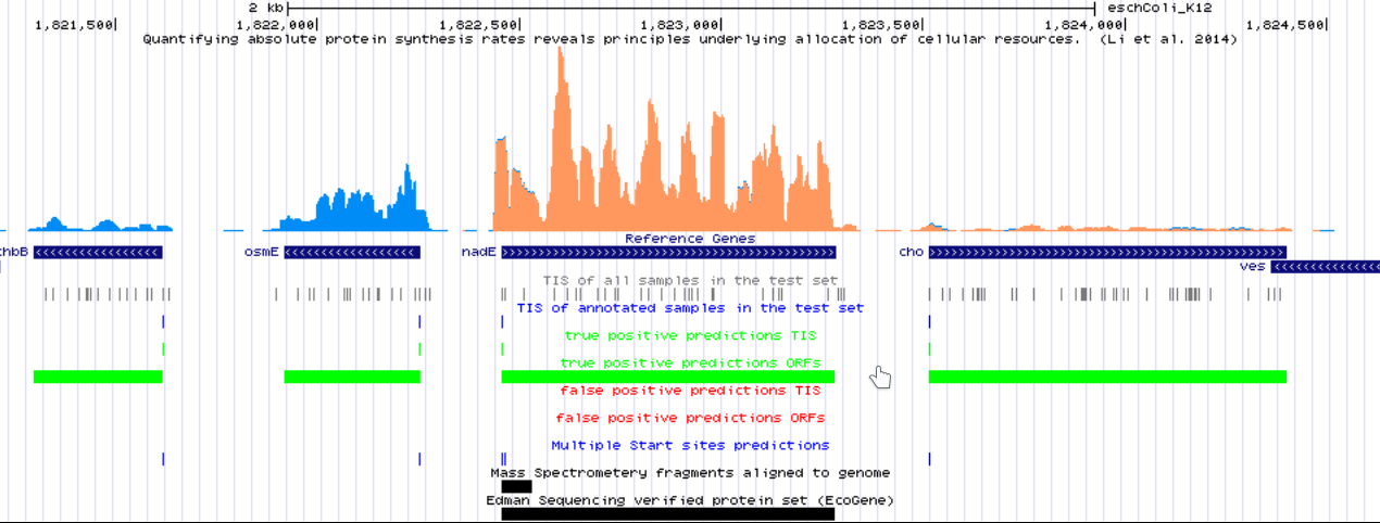
Created .bedgraph files are used to visualize the predictions of the model using a genome browser. This can be done using a local genome browser or even by using a UCSC hub. Annotations curated by DeepRibo to evaluate its performance can be browsed here. It is an example of how the annotations can be visualized using the hubs at GWIPS-viz.

Code Examples

These code examples will work with the data present if executed sequentially. The given data is incomplete and should be considered solely for the execution of these Code Examples.

parsing the data

Parsing E. coli, B. subtilis and S. typhimurium data:

python DataParser.py ../data/raw/eco_cov_sense.bedgraph ../data/raw/eco_cov_asense.bedgraph ../data/raw/eco_elo_sense.bedgraph ../data/raw/eco_elo_asense.bedgraph ../data/raw/eco.fa ../data/processed/ecoli -g ../data/raw/eco.gff -s ATG GTG TTG -p TAA TGA TAG

python DataParser.py ../data/raw/bac_cov_sense.bedgraph ../data/raw/bac_cov_asense.bedgraph ../data/raw/bac_elo_sense.bedgraph ../data/raw/bac_elo_asense.bedgraph ../data/raw/bac.fa ../data/processed/bacillus -g ../data/raw/bac.gff

python DataParser.py ../data/raw/sal_cov_sense.bedgraph ../data/raw/sal_cov_asense.bedgraph ../data/raw/sal_elo_sense.bedgraph ../data/raw/sal_elo_asense.bedgraph ../data/raw/sal.fa ../data/processed/salmonella -g ../data/raw/sal.gff

Training a model

python DeepRibo.py train ../data/processed --train_data ecoli salmonella --valid_size 0.3 -r 0 0 -c 0 0 --dest ../models/my_model -b 16 --GPU -v

DISCLAIMER : Normally the cut-off values can be obtained using the R script. Due to the small amount of mock data -r and -c are set at 0. In general, values are expected to be around -r 0.27 -c 0.12. A link to the complete datasets is given in the section Data. The flags for minimum RPKM -r and coverage -c have been given two sequential values, each given for the dataset listed by --train_data according to their shared order.

Predicting with a model

python DeepRibo.py predict ../data/processed --pred_data bacillus -r 0.0 -c 0.0 --model ../models/{MODEL NAME} --dest ../data/processed/bacillus/my_model_bac_pred.csv

Data

The complete datasets used to train and evaluate DeepRibo can be retrieved here. Most data has been retrieved from GWIPS-viz.

Changelog

Recent Major features implemented include:

• Updated code to work with Pytorch 1.4

• Added release tag

• PyTorch libraries updated from v0.3 to v0.4

• Implementation of custom neural network architectures

• A custom BucketSampler class, improving training times for large dataset up to 8 times

• Selection of start and stop triplets

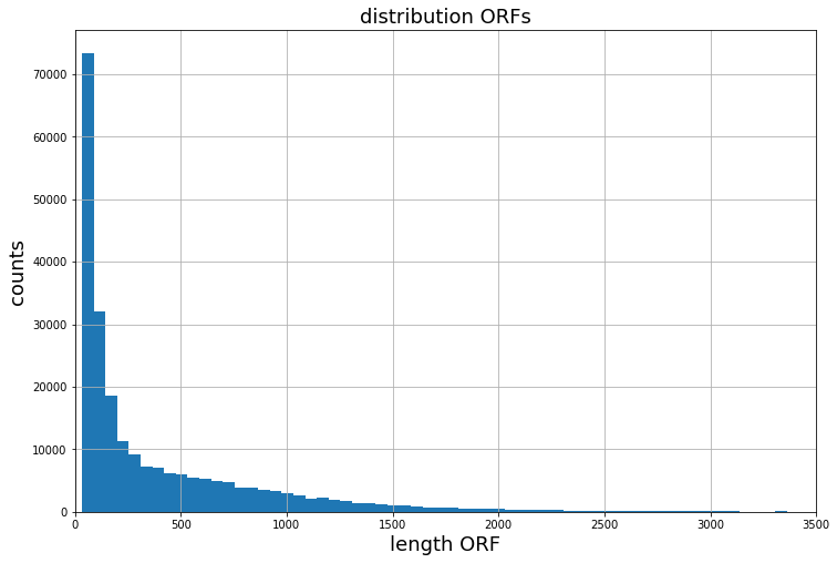
Given a typical distribution of ORFs lengths within a ribosome profiling experiment. Through bucketing, batches are created out of samples which share a similar length. When using random sampling, at least one long ORF is typically present within a batch, slowing the processing speed down significantly.