Slope failure under transient hydraulic loads

Authors: Veronica Girardi; Gaia Di Carluccio; Francesca Ceccato; Alba Yerro

In this tutorial, two typical macro-instabilities of water retaining geostructures are simulated with the two-phase formulation for unsaturated soils of Anura3D. The first mechanism, reported in Figure 1(a), is induced by a rapid draw-down, controlled by a transient total hydraulic head condition applied on the slope boundary. The second mechanism, reported in Figure 1(b), is triggered by a combination of high saturation of the slope body with an intense rainfall. In this case, rainfall and potential seepage face boundary conditions are applied on the slope.

Both cases are simulated in 2D-plane strain conditions. The $K_0$-procedure is used to expedite convergence during the first load step, where gravity is applied and quasi-static conditions considered. The $K_0$-procedure, when working with a problem in which the two-phase formulation for unsaturated soils is adopted, requires the user to specify:

• an initial soil surface
• an initial phreatic surface

The initial soil surface is selected by the user, after creating the slope geometry in GID. Whereas, the initial phreatic surface can be specified with one of two available methodologies: sketched by the user while creating the geometry in GID or assigned from an external file, which specifies the coordinates of two or more points associated to the phreatic surface location. It is also possible to initialize stresses using an input file in text format as explained in Section ??. After initialization, the two problems under analysis are modelled in fully dynamic conditions, applying respective hydraulic boundary conditions. Hence, failure and post-failure behaviors can be captured.

This tutorial demonstrates the use of

• two phase formulation for unsaturated soil;
• transient hydraulic boundary conditions (total head, rainfall and seepage face);
• stress initialization using $K_0$-procedure with the user-specified initial soil and phreatic surfaces. The latter can be either specified in the GID preprocessor or assigned considering an external file.
• Stress initialization by mean of an external text file.

Figure 12.1: Problem definition for failure of unsaturated slopes. Two mechanisms are analysed: an instability induced by rapid draw-down (a) and one triggered by the combination of high saturation and rainfall (b).

Problem definition

The slope geometry and the dimensions of the problem are given in Figure \ref{fig:unsatslope_dimensions}. The soil is modelled with the Mohr-Coulomb model and a linear SWRC with the properties given in the following Table.

Material type	unsaturated material - 2-phase with suction effects
initial porosity [-]	0.4
density solid [$kg/m^3$]	2650
density liquid [$kg/m^3$]	1000
intrinsic permeability liquid [$m^2$]	6e-12
Bulk modulus liquid [kPa]	60000
dynamic viscosity liquid [kPa s]	1e-6
$K_0$- value [-]	0.5
material model solid	Mohr-Coulomb
effective Poisson ratio [-]	0.3
effective Young modulus [kPa]	30000
effective cohesion [kPa]	1
effective friction angle [deg]	27
dilatancy angle [deg]	0.0
tensile strength [kPa]	0.0
liquid retention curve	linear
linear coefficient [1/kPa]	4e-4
hydraulic conductivity curve	constant

Rapid Drawdown

Creating input data

The geometry, discretization, material properties, and all other input parameters will be defined using the GiD pre-pocessor. This follows a similar procedure as described in Section \ref{chp:oedometer_problemdefinition}. Here only the differences with respect to previous examples will be highlighted.

Starting pre-processor

Start the GiD pre-processor following the steps as described in Section \ref{chp:oedometer_gid}. Set the problemtype as described in Section \ref{chp:oedometer_gid} step (2). Save the project in the desired directory with an appropriate name (e.g. "RapidDrawDown").

Defining units and dimensions

The problem is simulated in 2D-plane strain conditions; therefore, under \textit{Units and dimensions} in \textit{Problem dimensions}, select \textit{2D:plane-strain}. The single point formulation will be used; so, under \textit{Units and dimensions} in \textit{MPM discretization type}, select \textit{single_point}.

Defining geometry

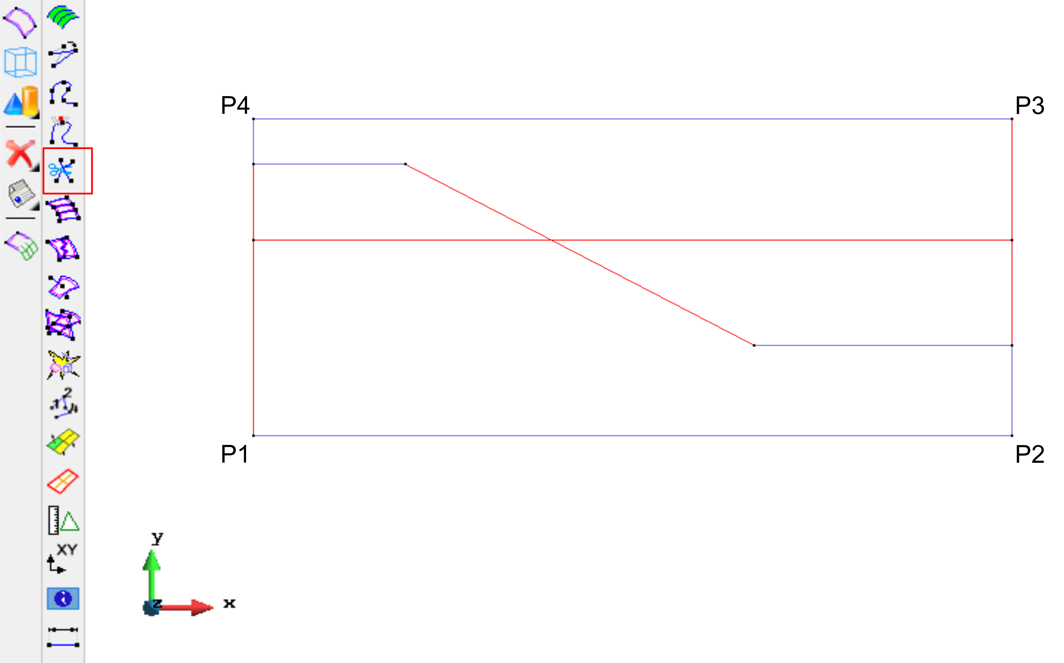
To generate the geometry follow the instructions given in Section \ref{chp:oedometer_geometry}. Figure \ref{fig:unsatslope_dimensions} reports the slope dimensions. The computational domain is extended vertically above the crest of the slope, the entire domain is bounded by four points of coordinates . The initial water table location corresponds to an horizontal line at y=2m. After drawing the line, the command \textit{Geometry create IntersectLine} is used to cut the lines intersected by the last line drawn. All these lines need to be selected (as displayed in Figure \ref{fig:unsatslope_lineCuts}) then press “esc” on your keyboard to obtain the final modification.

Figure 12.2: Lines definition with initial water table as a geometrical entity (line). Red lines are selected after using the command Geometry create IntersectLine.

Now it is possible to create the surfaces and complete the geometry definition, as visible in Figure

Figure 12.3: Geometry definition of the rapid draw down problem.

Define a new material with an appropriate name (e.g. "Slope") as explained in ??. Material parameters are given in Table 1.1 and shown in Figure 1.4, however during the initializa-tion phase two parameters are different: permeability should be assigned a value of

Figure 1.4: Defining material properties for the rapid draw down problem in GiD.

1.2.1.5 Specifying material points

Specify the initial material point distribution following instructions from Section ??. In this example choose 3 material points per element for the slope. Check if the material and the number of material points are assigned correctly (Figure1.5).

Figure 1.5: Specification of the material and number of material points per element in the rapid draw down problem.

1.2.1.6 Defining boundary conditions

Define the boundary conditions following the steps as described in Section ??.

Applying fixities
Since in this example a fully coupled two-phase analysis is performed, solid and liquid fixities must be assigned. The solid displacement at the boundaries will be fixed as follows:

(1) Left side: horizontal fixity in x-direction;
(2) Right side: horizontal fixity in x-direction;
(3) Top side: vertical fixity in y-direction;
(4) Bottom side: full fixities in x- and y-direction;
(5) Check if the x- and y- fixities are assigned correctly, see Figure 1.6;

Figure 1.6: Solid fixities for the rapid draw down problem.

The liquid displacement at the boundaries will be fixed as follows:

(1) Left side: horizontal fixity in x-direction;
(2) Right side: horizontal fixity in x-direction;
(3) Top side: vertical fixity in y-direction;
(4) Bottom side: vertical fixity in y-direction;
(5) Check if the x- and y- fixities are assigned correctly, see Figure 1.7;

Figure 1.7: Liquid fixities for the rapid draw down problem.

1.2.1.7 Defining initial conditions
The <img src="https://render.githubusercontent.com/render/math?math=\[

{width="5.709722222222222in" height="2.65in"}

Figure 1.8: Assign soil surface specification to lines for the rapid draw down problem.

The correct assignment can be verified by right-clicking on the option Soil Surface <img src="https://render.githubusercontent.com/render/math?math=\[

Figure 1.9: Checking the initial soil surface correct assignment for the rapid draw down model.

After specifying the soil surface, once more in the Anura3D menu under the section Initial con-
ditions, there is an option named Phreatic Surface <img src="https://render.githubusercontent.com/render/math?

Figure 1.10: Assign phreatic surface specification to lines for the rapid draw down prob- lem.

The correct assignment can be verified by right-clicking on the option Phreatic Surface <img src="https://render.githubusercontent.com/render/math?math=\[

Figure 1.11: Checking the initial phreatic surface correct assignment for the rapid draw down problem.

1.2.1.8 Defining hydraulic boundary conditions

The hydraulic boundary conditions, i.e. total hydraulic head, potential seepage face and rain-
fall, are assigned to boundary nodes of the body under analysis. Since the body is expected to
experience large displacements, initial boundary nodes may differ from boundary nodes at a
later stage of the simulation, thus it is necessary to define a potential area/volume of research
of boundary nodes, as explained in [? ]. This area is defined in GID, in the Anura3D menu, un-
der the section Boundary Conditions <img src="https://render.githubusercontent.com/render/math?math=\[

{width="5.1375in" height="2.3388877952755904in"}

Figure 1.12: Checking the assignment to the points defining the total hydraulic head po- tential area of research for the rapid draw down problem.

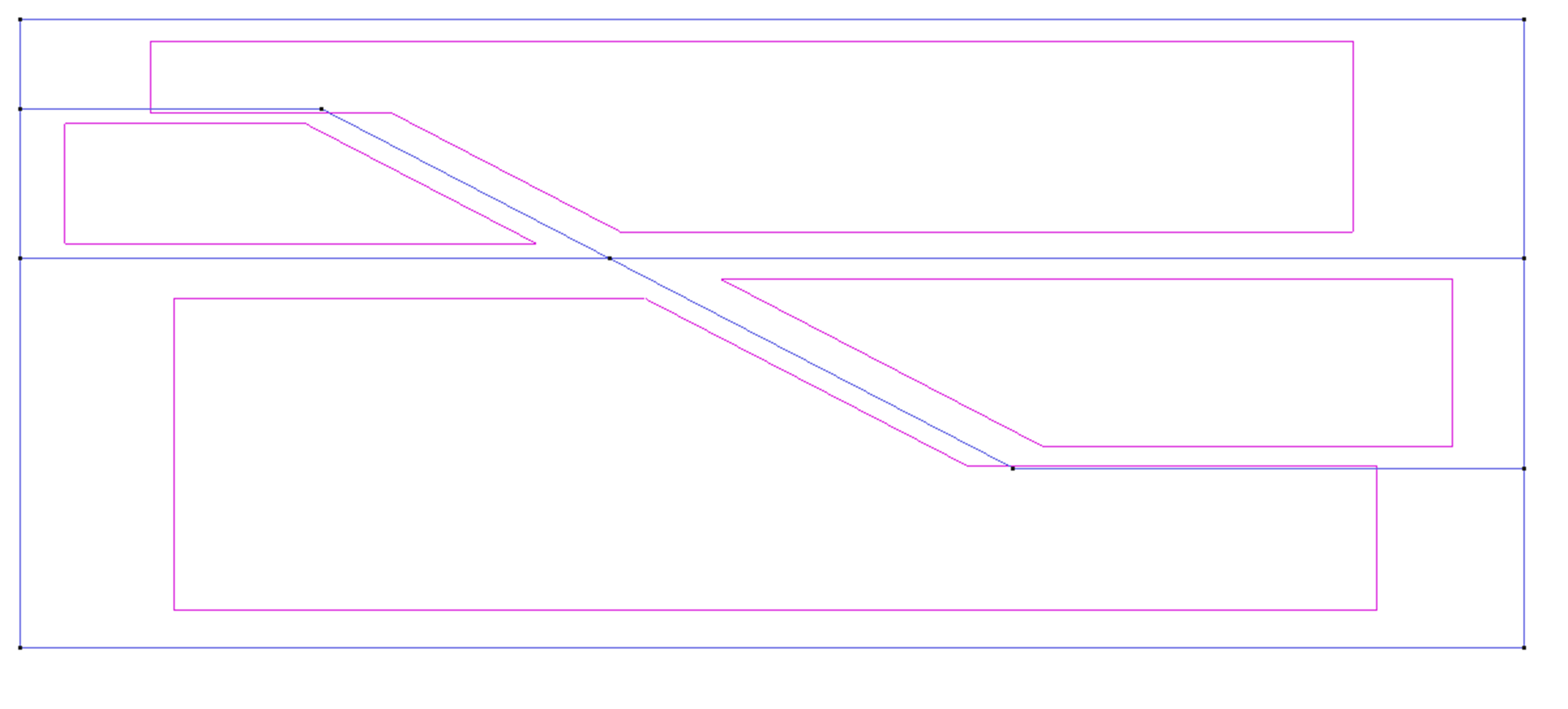
Here, it is possible to define for each hydraulic boundary condition, the coordinates of mini-mum and maximum points defining the rectangular area/ box volume where the condition is supposed to act for the entire simulation. In the rapid draw down problem it is necessary to as-sign an area to the total hydraulic head condition, and an equal area to the potential seepage face. In this manner, above the current river level (at the beginning of this simulation located at y=2m) the boundary condition applied to the slope is the potential seepage face. In GID under the selected hydraulic boundary condition, first double-click on x- and y- min and select the point P1. Click on <End> and <OK> for the correct assignment. Then, double-click on x-and y-max from the menu, select the point P3 (the points names are reported above in Figure 1.2), click on <End> and <OK>. The final assignment can be checked by right-clicking on Hy-draulic Head <img src="https://render.githubusercontent.com/render/math?math=\[The same procedure can be repeated, but this time the Seepage face condition should be selected in the menu. The final assignment should look as reported in Figure 1.13.

Figure 1.13: Checking the assignment to the points defining the seepage face potential area of research for the rapid draw down problem.

1.2.1.9 Creating mesh

An unstructured mesh is used for this example. To generate the mesh follow the steps given in Section ??. For this example the size assigned to all the surfaces is "0.4", and after click on Generate mesh, the size of elements to be generated should be set equal to 1. The mesh should count 552 triangular elements and 312 nodes as shown Figure 1.14.

{width="4.566666666666666in" height="2.0416666666666665in"}

Figure 1.14: Computational mesh of the rapid draw down problem.

The first load step is gravity loading, thus the input parameters are specific for this load step (Fig. ??). Section ?? explains how to modify the CPS for the following load steps.

Computation method
The option MPM - mixed integration should be selected.

Calculation step data
There is only 1 step for gravity loading. The end of the step is determined by the convergence criteria. A Courant number of 0.98 is advised to ensure the stability of the solution. Set number of calculation steps [-] to 1.

Gravity data
Use standard gravity value and unit vector down: <img src="https://render.githubusercontent.com/render/math?math

Gravity load
Gravity is applied from the beginning, therefore choose apply gravity load - stepwise and set the multipliers for gravity loading as 1.0 (initial and final value). The gravity multipliers will be maintained constant throughout the calculation.

Hydraulic head
In this example the total hydraulic head is applied, thus choose apply hydraulic head.

Seepage face
In this example the potential seepage face is applied, thus choose apply seepage face.

Quasi-static convergence
The end of the first load step is determined by convergence criteria, which corresponds to a quasi-static equilibrium condition. Set the QUASI-STATIC CONVERGENCE to apply con-vergence criteria . The convergence criteria are the tolerated error of the kinetic energy, the tolerated error of the out-of-balance force, or the maximum number of time steps. In this ex-ample, in order to reduce the computational time, use a maximum number of time steps equal to 2500.

Mass scaling
In this example the mass scaling is used to speed up the computation and a value of 80 is assigned to the mass scaling factor.

Homogeneous local damping
A local damping coefficient for all active elements of 0.05 is applied.

Strain smoothing
The strain smoothing algorithm will be switch on to minimise the kinematic locking.

Liquid pressure increment smoothing
The liquid pressure smoothing will be switch on to minimise pressure oscillations during the post-failure phase.