README.md

This website contains information regarding the paper Modular Flows: Differential Molecular Generation.

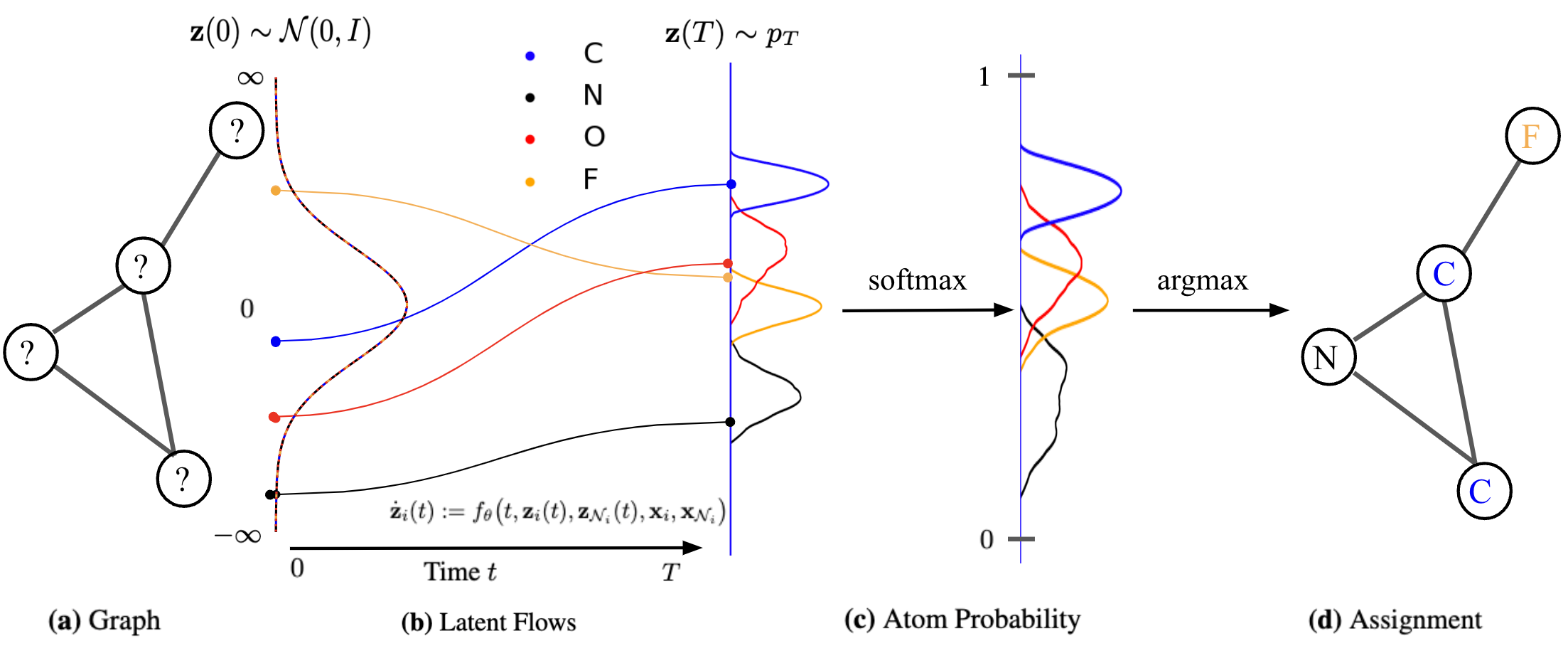
TL;DR: We propose generative graph normalizing flow models, based on a system of coupled node ODEs, that repeatedly reconcile locally toward globally aligned densities for high quality molecular generation

Please cite our work if you find it useful:

@misc{https://doi.org/10.48550/arxiv.2210.06032,
  doi = {10.48550/ARXIV.2210.06032},
  url = {https://arxiv.org/abs/2210.06032},
  author = {Verma, Yogesh and Kaski, Samuel and Heinonen, Markus and Garg, Vikas},
  keywords = {Machine Learning (cs.LG), Emerging Technologies (cs.ET), Biomolecules (q-bio.BM), Machine Learning (stat.ML), FOS: Computer and information sciences, FOS: Computer and information sciences, FOS: Biological sciences, FOS: Biological sciences},
  title = {Modular Flows: Differential Molecular Generation},
  publisher = {arXiv},
  year = {2022},
  copyright = {Creative Commons Attribution 4.0 International}
}

Problem of Molecular Generation

Generating new molecules is fundamental to advancing critical applications such as drug discovery and material synthesis. A key challenge of molecular generative models is to be able to generate valid molecules, according to various criteria for molecular validity or feasibility. It is a common practice to use external chemical software as rejection oracles to reduce or exclude invalid molecules, or do validity checks as part of autoregressive generation [1,2,3] . An important open question has been whether generative models can learn to achieve high generative validity intrinsically, i.e., without being aided by oracles or performing additional checks. We circumvent the issues with novel physics-inspired co-evolving continuous-time flows that induces useful inductive biases for a highly complex combinatorial setting. Our method is inspired by graph PDEs, that repeatedly reconcile locally toward globally aligned densities.

Continuous Normalizing Flows

Normalizing flow have seen widespread use for density modeling, generative modeling, etc which provides a general way of constructing flexible probability distributions. It is defined by a parameterized invertible deterministic transformation from a base distribution $$\mathcal{Z}$$ (e.g., Gaussian distribution) to real-world observational space $$X$$ (e.g. images and speech). When the dynamics of transformation is governed by an ODE, the method is known as Continous Normalizing Flows (CNFs). The process starts by sampling from a base distribution $$\mathbf{z}_0 \sim p_0(\mathbf{z}_0)$$, then solving the IVP $$\mathbf{z}(t_0) = \mathbf{z}_0$$, $$\dot{\mathbf{z}}(t) = \frac{\partial \mathbf{z}(t)}{\partial t} = f(\mathbf{z}(t),t;\theta)$$, where ODE is defined by the parametric function $$f(\mathbf{z}(t),t;\theta)$$ to obtain $$\mathbf{z}(t_1)$$ which constitutes our observable data. Then, using the instantaneous change of variables formula change in log-density under this model is given as:

$$\frac{\partial \log p_t(\mathbf{z}(t))}{\partial t} = -\texttt{tr} \left( \frac{\partial f}{\partial \mathbf{z}(t)} \right)$$

Given a datapoint $$\mathbf{x}$$, we can compute both the point $$\mathbf{z}{0}$$ which generates $$\mathbf{x}$$, as well as $$\log p_1(\mathbf{x})$$ by solving the initial value problem which integrates the combined dynamics of $$\mathbf{z}(t)$$ and the log-density of the sample resulting in the computation of $$\log p{1}(\mathbf{x})$$.

Modular Flows

Representation

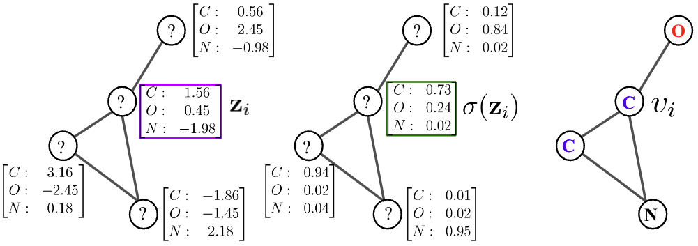
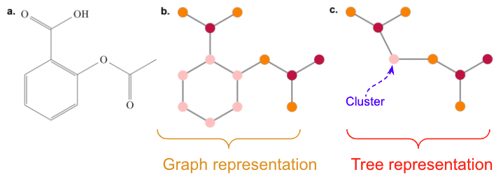
We represent molecule as a graph $$G = (V,E)$$, where each vertex takes value from an alphabet on atoms: $$v \in \mathcal{A} = { \texttt{C},\texttt{H},\texttt{N},\texttt{O},\texttt{P},\texttt{S},\ldots }$$; while the edges $$e \in \mathcal{B} = {1,2,3}$$ abstract the type of bond (i.e., single, double, or triple). We assume the following decomposition of the graph likelihood, over vertices conditioned on the edges and given the latent representations,

$$p(G) := p(V | E,\{ z\}) = \prod_{i=1}^M \texttt{Cat}(v_i | \sigma(\mathbf{z}_i))$$

We can obtain an alternative representation by decomposing a moleculer graph into a tree, by contracting certain vertices into a single node such that the molecular graph $$G$$ becomes acyclic. We followed a similar decompositon as JT-VAE[4], but restrict these clusters to ring-substructures, in addition to the atom alphabet. Thus, we obtain an extended alphabet vocabulary as $$\mathcal{A}{\mathrm{tree}} = { \texttt{C},\texttt{H},\texttt{N}, \ldots, \texttt{C}{1},\texttt{C}{2},\ldots }$$, where each cluster label $$\texttt{C}{r}$$ corresponds to the some ring-substructure in the label vocabulary $$\chi$$

Differential Modular Flows

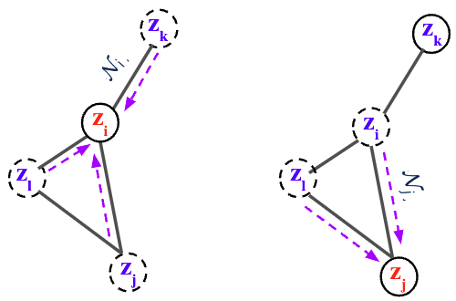
Based on the general recipie of normalizing flows, we propose to model the node scores $$\mathbf{z}{i}$$ as a Continuous-time Normalizing Flow (CNF)[7] over time $$t \in \mathrm{R}+$$. We assume the initial scores at time $$t=0$$ follow an uninformative Gaussian base distribution $$\mathbf{z}_i(0) \sim \mathcal{N}(0,I)$$ for each node $$i$$. Node scores evolve in parallel over time by a differential equation,

$$\dot{\mathbf{z}}_{i}(t) := \frac{\partial \mathbf{z}_i(t)}{\partial t} = f_\theta\big( t, \mathbf{z}_i(t), \mathbf{z}_{\mathcal{N}_i}(t),\mathbf{x}_{i}, \mathbf{x}_{\mathcal{N}_i} \big), \qquad i = 1, \ldots, M$$

where $$\mathcal{N}{i} = { \mathbf{z}{j} : (i,j) \in E }$$ is the set of neighbor scores at time $$t$$, $$\mathbf{x}$$ is the spatial information (2D/3D), and $$\theta$$ are the parameters of the flow function $$f$$ to be learned.

By collecting all node differentials we obtain a modular joint, coupled ODE, which is equivalent to a graph PDE [9,10], where the evolution of each node only depends on its immediate neighbors.

$$\dot{\mathbf{z}}_{i}(t) = \begin{pmatrix} \dot{\mathbf{z}}_{i}(t)_1(t) \\ \vdots \\ \dot{\mathbf{z}}_{i}(t)_M(t) \end{pmatrix} = \begin{pmatrix} f_\theta\big( t, \mathbf{z}_1(t), \mathbf{z}_{\mathcal{N}_1}(t),\mathbf{x}_{i}, \mathbf{x}_{\mathcal{N}_i} \big) \\ \vdots \\ f_\theta\big( t, \mathbf{z}_M(t), \mathbf{z}_{\mathcal{N}_M}(t),\mathbf{x}_{i}, \mathbf{x}_{\mathcal{N}_i} \big) \end{pmatrix} $$

## Equivariant local differential The goal is to have a function $$f_{\theta}$$ such that it satisfies natural equivariances and invariances of molecules like translation, rotational, reflection equivariances. Therefore, we chose to use E(3)-Equivariant GNN (EGNN)[11] which satisfies all the above criteria.

## Training Objective

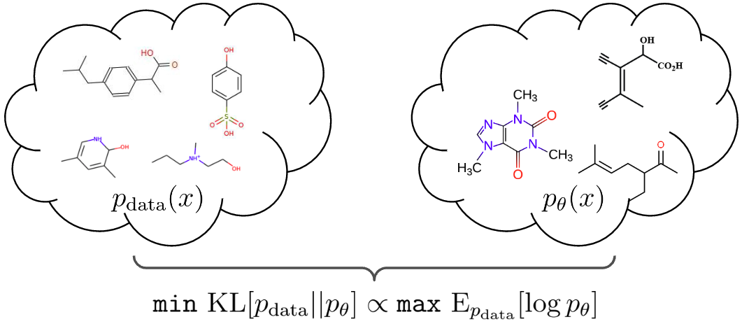
We reduce the learning problem to maximizing the score cross-entropy $$\mathrm{E}{\hat{p}{\mathrm{data}}(\mathbf{z}(T))}[\log p_\theta(\mathbf{z}(T))]$$, where we turn the observed set of graphs $${G_{n}}$$ into a set of scores $${\mathbf{z}_{n}}$$ by using one-hot encoding

$$\mathbf{z}_n (G_n; \epsilon) = (1-\epsilon)~\mathrm{onehot}(G_n) ~+~ \dfrac{\epsilon}{|\mathcal{A_s}|} \textbf{1}_{M(n)} \textbf{1}_{|\mathcal{A_s}|}^{\top}~,$$

where $$\mathrm{onehot}(G_{n})$$ is a matrix ($$M(n) \times |\mathcal{A_{s}}|$$), such that $$G_{n}(i, k)$$ = 1 if $$v_{i} = a_{k} \in \mathcal{A_{s}}$$, that is if the vertex $$i$$ is labeled with atom $$k$$, and 0 otherwise; $$\textbf{1}_{q}$$ is a vector with $$q$$ entries each set to 1; $$\mathcal{A_{s}} \in \{\mathcal{A}, \mathcal{A}_{\rm tree} \}$$; and $$\epsilon \in [0,1]$$ is added to model the noise in estimating the posterior $$p({\mathbf{z}(T)|G})$$. This is due to short-circuiting the inference process from $$G$$ to $$\mathbf{z}(T)$$ skipping the intermediate dependencies, as shown in the plate diagram.

We exploit the non-reversible composition of the argmax and softmax to transition from continous space to discrete graph space, but short-circuit in reverse direction as shown in the figure below. This indeed allows to keep the forward and backward flows aligned. We thus maximize an objective over $$N$$ training graphs,

$$\texttt{argmax}_\theta \qquad \mathcal{L} = \mathcal{E}_{\hat{p}_{\mathrm{data}}(\mathbf{z})} \log p_\theta(\mathbf{z}) \approx \frac{1}{N} \sum_{n=1}^N \log p_T\big( \mathbf{z}(T) = \mathbf{z}_n \big)$$

Molecule Generation

We generate novel molecules by sampling an initial state $$\mathbf{z}(0) \sim \mathcal{N}(0,I)$$ based on structure, and running the modular flow forward in time until $$\mathbf{z}(T)$$. This procedure maps a tractable base distribution $$p_0$$ to some more complex distribution $$p_T$$. We follow argmax to pick the most probable label assignment for each node as shown below.

Results

Density Estimation

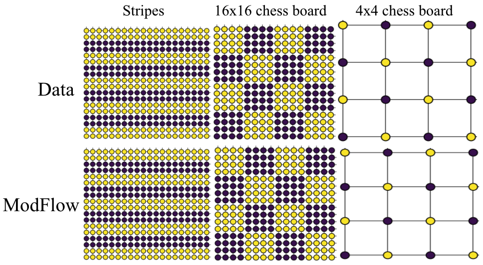
We demonstrated the power of our method on learning highly discontinous patterns on 2D grid graphs. We considered patterns corresponding to two-variants of chess-board pattern as $$4 \times 4$$, where every node has opposite value to its neighbors and $$16 \times 16$$ grid where blocks of $$4 \times 4$$ nodes have uniform values, but opposite across blocks. At last, we also considered alternate stripes pattern over $$20 \times 20$$ grid.

Molecular Experiments

We trained the model on QM9[6] and ZINC250K[5] dataset, where molecules are in kekulized form with hydrogens removed by the RDkit[8] software. We adopt common quality metrics to evaluate molecular generation as,

• Validity: Fraction of molecules that satisfy chemical valency rule
• Uniqueness: Fraction of non-duplicate generations
• Novelty: Fraction of molecules not present in training data
• Reconstruction: Fraction of molecules that can be reconstructed from their encoding

Apart from these metrics, we also evaluated our method on MOSES metrics. These are:

• FCD: measures diversity and chemical and biological property alignment
• SNN: quantifies closeness of generated molecules to true molecule manifold
• Frag: measures distance between the fragment frequencies generated and reference
• IntDiv: diversity by computing pairwise similarity of the generated molecules

Some of the generated molecules via $$\texttt{ModFlow}$$ are also shown above. We visually evaluate the generated structures via out method via properties distribution. We utilize kernel density estimation of these distributions to visualize these distributions. We use

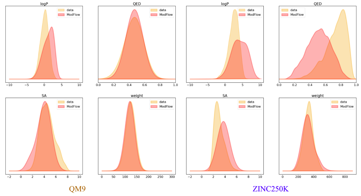
• Molecular Weight: Sum of the individual atomic weights of a molecule.
• LogP: Ratio of concentration in octanol-phase to aqueous phase, also known as the octanol-water partition coefficient.
• Synthetic Accessibility Score (SA): Estimate describing the synthesizability of a given molecule
• Quantitative Estimation of Drug-likeness (QED): Value describing likeliness of a molecule as a viable candidate for a drug

Property-targeted Molecular Optimization

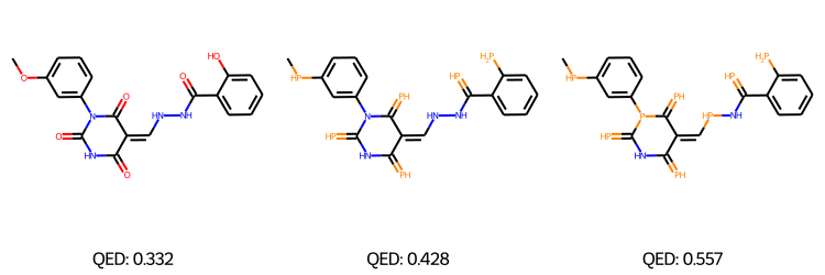
We performed Property-targeted Molecular Optimization, to search for molecules, having a better chemical properties. Specifically, we choose quantitative estimate of drug-likeness (QED) as our target chemical property, which measures the potential of a molecule to be characterized as a drug. We used a pre-trained ModFlow model $$f$$, to encode a molecule $$\mathcal{M}$$ and get the embedding $$Z = f(\mathcal{M})$$, and further used linear regression to regress these embeddings to the QED scores and interpolated in the latent space space of a molecule along the direction of increasing QED. This is done via gradient ascend method, $$Z' = Z + \lambda*\frac{dy}{dZ}$$ where $$y$$ is the QED score and $$\lambda$$ is the length of the search step. The above method is conducted for $$K$$ steps, and the new embedding $$Z'$$ is decoded back to molecule space via reverse mapping $$\mathcal{M}' = f^{-1}(\mathcal{Z}')$$.

The above figures represent the molecules decoded from the learned latent space with linear regression for successful molecular optimization.

Ablation Studies

We performed ablation experiments to gain further insights about $$\texttt{ModFlow}$$. Specifically, we conducted ablation study to quantify the effect of incorporating the symmetries in our model as E(3) Equivariant vs Not Equivariant, where we compare the results to a 3-layer GCN and investigated whether including 3D coordinate information 2D vs 3D, improves the model and evaluate the benefit of including the geometric information.

Conclusion

1. We propose Physics-inspired co-evolving continuous-time flows, inspired by graph PDEs as $$\texttt{ModFlow}$$, where multiple flows interact locally according to a modular coupled ODE system.
2. The coupled dynamics results in accurate modeling of graph densities and high quality molecular generation without any validity checks or correction.
3. Interesting avenues open up, including the design of (a) more nuanced mappings between discrete and continuous spaces, and (b) extensions of modular flows to (semi-)supervised settings.

References

1. Youzhi Luo, Keqiang Yan, and Shuiwang Ji. Graphdf: A discrete flow model for molecular graph generation,2021
2. Chence Shi, Minkai Xu, Zhaocheng Zhu, Weinan Zhang, Ming Zhang, and Jian Tang. Graphaf: a flow-based autoregressive model for molecular graph generation
3. Mariya Popova, Mykhailo Shvets, Junier Oliva, and Olexandr Isayev. Molecularrnn: Generating realistic molecular graphs with optimized properties,2019
4. Wengong Jin, Regina Barzilay, and Tommi Jaakkola. Junction tree variational autoencoder for molecular graph generation
5. John J Irwin, Teague Sterling, Michael M Mysinger, Erin S Bolstad, and Ryan G Coleman. Zinc: a free tool to discover chemistry for biology. Journal of chemical information and modeling, 52(7):1757–1768, 2012
6. Raghunathan Ramakrishnan, Pavlo O Dral, Matthias Rupp, and O Anatole von Lilienfeld. Quantum chemistry structures and properties of 134 kilo molecules. Scientific Data, 1, 2014
7. Will Grathwohl, Ricky TQ Chen, Jesse Bettencourt, Ilya Sutskever, and David Duvenaud. Ffjord: Free-form continuous dynamics for scalable reversible generative models
8. Greg Landrum et al. Rdkit: A software suite for cheminformatics, computational chemistry, and predictive modeling, 2013
9. Valerii Iakovlev, Markus Heinonen, and Harri Lähdesmäki. Learning continuous-time pdes from sparse data with graph neural networks.
10. Ben Chamberlain, James Rowbottom, Maria I Gorinova, Michael Bronstein, Stefan Webb, and Emanuele Rossi Grand: Graph neural diffusion. In International Conference on Machine Learning, pages 1407–1418. PMLR, 2021
11. Victor Garcia Satorras, Emiel Hoogeboom, and Max Welling. E(n) equivariant graph neural networks, 2021