Home
The following details the steps involved in:
- Generating a Trinity de novo RNA-Seq assembly
- Evaluating the quality of the assembly
- Quantifying transcript expression levels
- Identifying differentially expressed (DE) transcripts
- Functionally annotating transcripts using Trinotate and predicting coding regions using TransDecoder
- Examining functional enrichments for DE transcripts using GOseq
- Interactively Exploring annotations and expression data via TrinotateWeb
All required software and data are provided pre-installed on the Amazon EC2 AMI 'ami-2f6f3445'. Be sure to have a running instance on at least an m3.large instance type, so we'll have adequate computational resources allocated in addition to reasonable response times over the network.
The workshop materials here expect that you have a minimal familiarity with UNIX.
After launching and connecting to your running instance of the AMI, change your working directory to the base directory of these workshop materials. We'll get there by moving down three directories:
    %  cd workshop_data

    %  cd transcriptomics

    %  cd KrumlovTrinityWorkshopJan2016
Yes, you could have just 'cd workshop_data/transcriptomics/KrumlovTrinityWorkshopJan2016', but here we're taking the slower scenic route. Feel free to look around and run 'ls' to see what other files or directories are there along the way and get a feel for where you are in the file system - which is particularly useful if you're new to unix.
This 'KrumlovTrinityWorkshopJan2016' will be the base working directory for all the exercises below. We'll create other subdirectories here and move back and forth to our various workspaces that we generate along the way.
Below, we refer to '%' as the terminal command prompt, and we use environmental variables such as $TRINITY_HOME and $TRINOTATE_HOME as shortcuts to referring to their installation directories in the AMI image. To view the path to the installation directories, you can simply run:
% echo $TRINITY_HOME
Also, some commands can be fairly long to type in, an so they'll be more easily displayed in this document, we separate parts of the command with '' characters and put the rest of the command on the following line. Similarly in unix you can type '[return]' and you can continue to type in the rest of the command on the new line in the terminal.
For viewing text files, we'll use the unix utilities 'head' (look at the top few lines), 'cat' (print the entire contents of the file), and 'less' (interactively page through the file), and for viewing PDF formatted files, we'll use the 'xpdf' viewer utility.
Because the workshop materials have been tweaked ever so slightly after we had built the final AMI, we'll need to update the materials in this workshop data space to capture the latest content.
To update, run the following two commands:
% rm data/mini_sprot.pep

% git pull
Assuming no fatal errors occurred, you should now be ready for running the exercises below.
For this course we will be using the data from this paper: Defining the transcriptomic landscape of Candida glabrata by RNA-Seq. Linde et al. Nucleic Acids Res. 2015 This work provides a detailed RNA-Seq-based analysis of the transcriptomic landscape of C. glabrata in nutrient-rich media (WT), as well as under nitrosative stress (GSNO), in addition to other conditions, but we'll restrict ourselves to just WT and GSNO conditions for demonstration purposes in this workshop.
There are paired-end FASTQ formatted Illlumina read files for each of the two conditions, with three biological replicates for each. All RNA-Seq data sets can be found in the data/ subdirectory:
% ls -1 data | grep fastq
.
GSNO_SRR1582646_1.fastq
GSNO_SRR1582646_2.fastq
GSNO_SRR1582647_1.fastq
GSNO_SRR1582647_2.fastq
GSNO_SRR1582648_1.fastq
GSNO_SRR1582648_2.fastq
wt_SRR1582649_1.fastq
wt_SRR1582649_2.fastq
wt_SRR1582650_1.fastq
wt_SRR1582650_2.fastq
wt_SRR1582651_1.fastq
wt_SRR1582651_2.fastq
Each biological replicate (eg. wt_SRR1582651) contains a pair of fastq files (eg. wt_SRR1582651_1.fastq.gz for the 'left' and wt_SRR1582651_2.fastq.gz for the 'right' read of the paired end sequences). Normally, each file would contain millions of reads, but in order to reduce running times as part of the workshop, each file provided here is restricted to only 10k RNA-Seq reads.
It's generally good to evaluate the quality of your input data using a tool such as FASTQC. Since exploration of FASTQC reports has already been done in a previous section of this workshop, we'll skip doing it again here - and trust that the quality of these reads meet expectations.
Finally, another set of files that you will find in the data include 'mini_sprot.pep*', corresponding to a highly abridged version of the SWISSPROT database, containing only the subset of protein sequences that are needed for use in this workshop. It's provided and used here only to speed up certain operations, such as BLAST searches, which will be performed at several steps in the tutorial below. Of course, in exploring your own RNA-Seq data, you would leverage the full version of SWISSPROT and not this tiny subset used here.
To generate a reference assembly that we can later use for analyzing differential expression, we'll combine the read data sets for the different conditions together into a single target for Trinity assembly. We do this by providing Trinity with a list of all the left and right fastq files to the --left and --right parameters as comma-delimited like so:
   %   ${TRINITY_HOME}/Trinity --seqType fq  \
           --left data/wt_SRR1582649_1.fastq,data/wt_SRR1582651_1.fastq,data/wt_SRR1582650_1.fastq,data/GSNO_SRR1582648_1.fastq,data/GSNO_SRR1582646_1.fastq,data/GSNO_SRR1582647_1.fastq \
          --right data/wt_SRR1582649_2.fastq,data/wt_SRR1582651_2.fastq,data/wt_SRR1582650_2.fastq,data/GSNO_SRR1582648_2.fastq,data/GSNO_SRR1582646_2.fastq,data/GSNO_SRR1582647_2.fastq \
          --CPU 2 --max_memory 2G --min_contig_length 150
Note, if you see a message about not being able to identify the version of Java, please just ignore it.
Running Trinity on this data set may take 10 to 15 minutes. You'll see it progress through the various stages, starting with Jellyfish to generate the k-mer catalog, then followed by Inchworm to assemble 'draft' contigs, Chrysalis to cluster the contigs and build de Bruijn graphs, and finally Butterfly for tracing paths through the graphs and reconstructing the final isoform sequences.
Running a typical Trinity job requires ~1 hour and ~1G RAM per ~1 million PE reads. You'd normally run it on a high-memory machine and let it churn for hours or days.
The assembled transcripts will be found at 'trinity_out_dir/Trinity.fasta'.
Just to look at the top few lines of the assembled transcript fasta file, you can run:
% head trinity_out_dir/Trinity.fasta
and you can see the Fasta-formatted Trinity output:
>TRINITY_DN506_c0_g1_i1 len=171 path=[149:0-170] [-1, 149, -2]
TGAGTATGGTTTTGCCGGTTTGGCTGTTGGTGCAGCTTTGAAGGGCCTAAAGCCAATTGT
TGAATTCATGTCATTCAACTTCTCCATGCAAGCCATTGACCATGTCGTTAACTCGGCAGC
AAAGACACATTATATGTCTGGTGGTACCCAAAAATGTCAAATCGTGTTCAG
>TRINITY_DN512_c0_g1_i1 len=168 path=[291:0-167] [-1, 291, -2]
ATATCAGCATTAGACAAAAGATTGTAAAGGATGGCATTAGGTGGTCGAAGTTTCAGGTCT
AAGAAACAGCAACTAGCATATGACAGGAGTTTTGCAGGCCGGTATCAGAAATTGCTGAGT
AAGAACCCATTCATATTCTTTGGACTCCCGTTTTGTGGAATGGTGGTG
>TRINITY_DN538_c0_g1_i1 len=310 path=[575:0-309] [-1, 575, -2]
GTTTTCCTCTGCGATCAAATCGTCAAACCTTAGACCTAGCTTGCGGTAACCAGAGTACTT
Note, the sequences you see will likely be different, as the order of sequences in the output is not deterministic.
The FASTA sequence header for each of the transcripts contains the identifier for the transcript (eg. 'TRINITY_DN506_c0_g1_i1'), the length of the transcript, and then some information about how the path was reconstructed by the software by traversing nodes within the graph.
It is often the case that multiple isoforms will be reconstructed for the same 'gene'. Here, the 'gene' identifier corresponds to the prefix of the transcript identifier, such as 'TRINITY_DN506_c0_g1', and the different isoforms for that 'gene' will contain different isoform numbers in the suffix of the identifier (eg. TRINITY_DN506_c0_g1_i1 and TRINITY_DN506_c0_g1_i2 would be two different isoform sequences reconstructed for the single gene TRINITY_DN506_c0_g1). It is useful to perform certain downstream analyses, such as differential expression, at both the 'gene' and at the 'isoform' level, as we'll do later below.
There are several ways to quantitatively as well as qualitatively assess the overall quality of the assembly, and we outline many of these methods at our Trinity wiki.
You can count the number of assembled transcripts by using 'grep' to retrieve only the FASTA header lines and piping that output into 'wc' (word count utility) with the '-l' parameter to just count the number of lines.
% grep '>' trinity_out_dir/Trinity.fasta | wc -l
How many were assembled?
It's useful to know how many transcript contigs were assembled, but it's not very informative. The deeper you sequence, the more transcript contigs you will be able to reconstruct. It's not unusual to assemble over a million transcript contigs with very deep data sets and complex transcriptomes, but as you 'll see below (in the section containing the more informative guide to assembly assessment) a fraction of the transcripts generally best represent the input RNA-Seq reads.
Capture some basic statistics about the Trinity assembly:
% $TRINITY_HOME/util/TrinityStats.pl trinity_out_dir/Trinity.fasta
which should generate data like so. Note your numbers may vary slightly, as the assembly results are not deterministic.
################################
## Counts of transcripts, etc.
################################
Total trinity 'genes':	695
Total trinity transcripts:	695
Percent GC: 44.43

########################################
Stats based on ALL transcript contigs:
########################################

Contig N10: 656
Contig N20: 511
Contig N30: 420
Contig N40: 337
Contig N50: 284

Median contig length: 214
Average contig: 274.44
Total assembled bases: 190738


#####################################################
## Stats based on ONLY LONGEST ISOFORM per 'GENE':
#####################################################

Contig N10: 656
Contig N20: 511
Contig N30: 420
Contig N40: 337
Contig N50: 284

Median contig length: 214
Average contig: 274.44
Total assembled bases: 190738
The total number of reconstructed transcripts should match up identically to what we counted earlier with our simple 'grep | wc' command. The total number of 'genes' is also reported - and simply involves counting up the number of unique transcript identifier prefixes (without the _i isoform numbers). When the 'gene' and 'transcript' identifiers differ, it's due to transcripts being reported as alternative isoforms for the same gene. In our tiny example data set, we unfortunately do not reconstruct any alternative isoforms, and note that alternative splicing in this yeast species may be fairly rare. Tackling an insect or mammal transcriptome would be expected to yeild many alternative isoforms.
You'll also see 'Contig N50' values reported. You'll remmeber from the earlier lectures on genome assembly that the 'N50 statistic indicates that at least half of the assembled bases are in contigs of at least that contig length'. We extend the N50 statistic to provide N40, N30, etc. statistics with similar meaning. As the N-value is decreased, the corresponding length will increase.
Most of this is not quantitatively useful, and the values are only reported for historical reasons - it's simply what everyone used to do in the early days of transcriptome assembly. The N50 statistic in RNA-Seq assembly can be easily biased in the following ways:
-
Overzealous reconstruction of long alternatively spliced isoforms: If an assembler tends to generate many different 'versions' of splicing for a gene, such as in a combinatorial way, and those isoforms tend to have long sequence lengths, the N50 value will be skewed towards a higher value.
-
Highly sensitive reconstruction of lowly expressed isoforms: If an assembler is able to reconstruct transcript contigs for those transcirpts that are very lowly expressed, these contigs will tend to be short and numerous, biasing the N50 value towards lower values. As one sequences deeper, there will be more evidence (reads) available to enable reconstruction of these short lowly expressed transcripts, and so deeper sequencing can also provide a downward skew of the N50 value.
We now move into the section containing more meaningful metrics for evaluating your transcriptome assembly.
A high quality transcriptome assembly is expected to have strong representation of the reads input to the assembler. By aligning the RNA-Seq reads back to the transcriptome assembly, we can quantify read representation. In Trinity, we have a script that will align each of the fastq files of the paired read set to the assembly separately, and then link up the pairs. This way, we can count the number of reads that are found as properly paired alignments in addition to those that align to separate contigs (improperly paired), in addition to those cases where only one of the paired reads (the left or the right read of the pair) aligns to a contig. Run the following, which wraps the Bowtie software to do the read alignments:
%  $TRINITY_HOME/util/bowtie_PE_separate_then_join.pl \
      --target trinity_out_dir/Trinity.fasta \
      --seqType fq \
      --left data/wt_SRR1582651_1.fastq \
      --right data/wt_SRR1582651_2.fastq \
      --aligner bowtie -- -p 2 --all --best --strata -m 300
The output files will exist in a bowtie_out/ subdirectory. You can look at the list of files generated like so:
% ls -ltr bowtie_out/
Among the outputs, you should find a name-sorted bam file (where aligned reads are sorted by their name, instead of by their coordinate) called 'bowtie_out/bowtie_out.nameSorted.bam'. Using this file and another script in the Trinity software suite, we can count the number of reads that correspond to the different alignment categories:
%  $TRINITY_HOME/util/SAM_nameSorted_to_uniq_count_stats.pl \
       bowtie_out/bowtie_out.nameSorted.bam
.
#read_type	count	pct
improper_pairs	3552	50.40
proper_pairs	2580	36.61
right_only	527	7.48
left_only	388	5.51

Total aligned reads: 7047
Generally, in a high quality assembly, you would expect to see at least ~70% and at least ~70% of the reads to exist as proper pairs. Our tiny read set used here in this workshop does not provide us with a high quality assembly, as only 36% of aligned reads are mapped as proper pairs, and half of aligned reads (50%) are found as 'improper_pairs', indicating that both paired reads align to the assembly, but they align to different transcript contigs - which is usually the sign of a fractured assembly. In this case, deeper sequencing and assembly of more reads would be expected to lead to major improvements here.
Another very useful metric in evaluating your assembly is to assess the number of fully reconstructed coding transcripts. This can be done by performing a BLASTX search of your assembled transcript sequences to a high quality database of protein sequences, such as provided by SWISSPROT. Searching a large protein database using BLASTX can take a while - longer than we want during this workshop, so instead, we'll search the mini-version of SWISSPROT that comes installed in our data/ directory:
% blastx -query trinity_out_dir/Trinity.fasta \
         -db data/mini_sprot.pep -out blastx.outfmt6 \
         -evalue 1e-20 -num_threads 2 -max_target_seqs 1 -outfmt 6
The above blastx command will have generated an output file 'blastx.outfmt6', storing only the single best matching protein given the E-value threshold of 1e-20. By running another script in the Trinity suite, we can compute the length representation of best matching SWISSPROT matches like so:
% $TRINITY_HOME/util/analyze_blastPlus_topHit_coverage.pl \
       blastx.outfmt6 trinity_out_dir/Trinity.fasta \
       data/mini_sprot.pep | column -t
.
#hit_pct_cov_bin  count_in_bin  >bin_below
100               77            77
90                18            95
80                12            107
70                17            124
60                16            140
50                24            164
40                34            198
30                43            241
20                64            305
10                24            329
The above table lists bins of percent length coverage of the best matching protein sequence along with counts of proteins found within that bin. For example, 77 proteins are matched by more than 90% of their length up to 100% of their length. There are 18 matched by more than 80% and up to 90% of their length. The third column provides a running total, indicating that 95 transcripts match more than 80% of their length, and 107 transcripts match more than 70% of their length, etc.
The count of full-length transcripts is going to be dependent on how good the assembly is in addition to the depth of sequencing, but should saturate at higher levels of sequencing. Performing this full-length transcript analysis using assemblies at different read depths and plotting the number of full-length transcripts as a function of sequencing depth will give you an idea of whether or not you've sequenced deeply enough or you should consider doing more RNA-Seq to capture more transcripts and obtain a better (more complete) assembly.
We'll explore some additional metrics that are useful in assessing the assembly quality below, but they require that we estimate expression values for our transcripts, so we'll tackle that first.
To estimate the expression levels of the Trinity-reconstructed transcripts, we use the strategy supported by the RSEM software involving read alignment followed by expectation maximization to assign reads according to maximum likelihood estimates. In essence, we first align the original rna-seq reads back against the Trinity transcripts, then run RSEM to estimate the number of rna-seq fragments that map to each contig. Because the abundance of individual transcripts may significantly differ between samples, the reads from each sample (and each biological replicate) must be examined separately, obtaining sample-specific abundance values.
We include a script to faciliate running of RSEM on Trinity transcript assemblies. The script we execute below will run the Bowtie aligner to align reads to the Trinity transcripts, and RSEM will then evaluate those alignments to estimate expression values. Again, we need to run this separately for each sample and biological replicate (ie. each pair of fastq files).
Let's start with one of the GSNO treatment fastq pairs like so:
 %  $TRINITY_HOME/util/align_and_estimate_abundance.pl --seqType fq \
         --left data/GSNO_SRR1582648_1.fastq \
         --right data/GSNO_SRR1582648_2.fastq  \
         --transcripts trinity_out_dir/Trinity.fasta  \
         --output_prefix GSNO_SRR1582648 \
         --est_method RSEM  --aln_method bowtie \
         --trinity_mode --prep_reference --coordsort_bam \
         --output_dir GSNO_SRR1582648.RSEM
The outputs generated from running the command above will exist in the GSNO_SRR1582648.RSEM/ directory, as we indicate with the --output_dir parameter above.
The primary output generated by RSEM is the file containing the expression values for each of the transcripts. Examine this file like so:
% head GSNO_SRR1582648.RSEM/GSNO_SRR1582648.isoforms.results | column -t
and you should see the top of a tab-delimited file:
transcript_id           gene_id              length  effective_length  expected_count  TPM      FPKM      IsoPct
TRINITY_DN0_c0_g1_i1    TRINITY_DN0_c0_g1    328     198.75            29.00           9093.16  43883.19  100.00
TRINITY_DN0_c0_g2_i1    TRINITY_DN0_c0_g2    329     199.75            0.00            0.10     0.48      100.00
TRINITY_DN100_c0_g1_i1  TRINITY_DN100_c0_g1  198     69.79             1.00            892.99   4309.53   100.00
TRINITY_DN101_c0_g1_i1  TRINITY_DN101_c0_g1  233     104.12            2.00            1197.08  5777.04   100.00
TRINITY_DN102_c0_g1_i1  TRINITY_DN102_c0_g1  198     69.79             0.00            0.00     0.00      0.00
TRINITY_DN103_c0_g1_i1  TRINITY_DN103_c0_g1  346     216.72            7.00            2012.95  9714.40   100.00
TRINITY_DN104_c0_g1_i1  TRINITY_DN104_c0_g1  264     134.91            1.00            461.94   2229.29   100.00
TRINITY_DN105_c0_g1_i1  TRINITY_DN105_c0_g1  540     410.62            19.00           2883.65  13916.35  100.00
TRINITY_DN106_c0_g1_i1  TRINITY_DN106_c0_g1  375     245.67            3.00            761.01   3672.58   100.00
The key columns in the above RSEM output are the transcript identifier, the 'expected_count' corresponding to the number of RNA-Seq fragments predicted to be derived from that transcript, and the 'TPM' or 'FPKM' columns, which provide normalized expression values for the expression of that transcript in the sample.
The FPKM expression measurement normalizes read counts according to the length of transcripts from which they are derived (as longer transcripts generate more reads at the same expression level), and normalized according to sequencing depth. The FPKM acronym stand for 'fragments per kilobase of cDNA per million fragments mapped'.
TPM 'transcripts per million' is generally the favored metric, as all TPM values should sum to 1 million, and TPM nicely reflects the relative molar concentration of that transcript in the sample. FPKM values, on the other hand, do not always sum to the same value, and do not have the similar property of inherrently representing a proportion within a sample, making comparisons between samples less straightforward. TPM values can be easily computed from FPKM values like so: TPMi = FPKMi / (sum all FPKM values) * 1 million.
Note, a similar RSEM outputted gene expression file exists for the 'gene' level expression data. For example:
% head GSNO_SRR1582648.RSEM/GSNO_SRR1582648.genes.results | column -t
.
gene_id              transcript_id(s)        length  effective_length  expected_count  TPM      FPKM
TRINITY_DN0_c0_g1    TRINITY_DN0_c0_g1_i1    328.00  198.75            29.00           9093.16  43883.19
TRINITY_DN0_c0_g2    TRINITY_DN0_c0_g2_i1    329.00  199.75            0.00            0.10     0.48
TRINITY_DN100_c0_g1  TRINITY_DN100_c0_g1_i1  198.00  69.79             1.00            892.99   4309.53
TRINITY_DN101_c0_g1  TRINITY_DN101_c0_g1_i1  233.00  104.12            2.00            1197.08  5777.04
TRINITY_DN102_c0_g1  TRINITY_DN102_c0_g1_i1  198.00  69.79             0.00            0.00     0.00
TRINITY_DN103_c0_g1  TRINITY_DN103_c0_g1_i1  346.00  216.72            7.00            2012.95  9714.40
TRINITY_DN104_c0_g1  TRINITY_DN104_c0_g1_i1  264.00  134.91            1.00            461.94   2229.29
TRINITY_DN105_c0_g1  TRINITY_DN105_c0_g1_i1  540.00  410.62            19.00           2883.65  13916.35
TRINITY_DN106_c0_g1  TRINITY_DN106_c0_g1_i1  375.00  245.67            3.00            761.01   3672.58
Running this on all the samples can be montonous, and with many more samples, advanced users would generally write a short script to fully automate this process. We won't be scripting here, but instead just directly execute abundance estimation just as we did above but on the other five pairs of fastq files. We'll examine the outputs of each in turn, as a sanity check and also just for fun.
Process fastq pair 2:
 % $TRINITY_HOME/util/align_and_estimate_abundance.pl --seqType fq  \
         --left data/GSNO_SRR1582646_1.fastq \
         --right data/GSNO_SRR1582646_2.fastq \
         --transcripts trinity_out_dir/Trinity.fasta \
         --output_prefix GSNO_SRR1582646 \
         --est_method RSEM  --aln_method bowtie \
         --trinity_mode --prep_reference --coordsort_bam  \
         --output_dir GSNO_SRR1582646.RSEM
Process fastq pair 3:
 % $TRINITY_HOME/util/align_and_estimate_abundance.pl --seqType fq \
    --left data/GSNO_SRR1582647_1.fastq \
    --right data/GSNO_SRR1582647_2.fastq \
    --transcripts trinity_out_dir/Trinity.fasta  \
    --output_prefix GSNO_SRR1582647 \
    --est_method RSEM --aln_method bowtie --trinity_mode \
    --prep_reference --coordsort_bam  \
    --output_dir GSNO_SRR1582647.RSEM
Now we're done with processing the GSNO-treated biological replicates, and we'll proceed to now run abundance estimations for the WT samples.
Process fastq pair 4:
 % $TRINITY_HOME/util/align_and_estimate_abundance.pl --seqType fq \
     --left data/wt_SRR1582649_1.fastq \
     --right data/wt_SRR1582649_2.fastq \
     --transcripts trinity_out_dir/Trinity.fasta \
     --output_prefix wt_SRR1582649 \
     --est_method RSEM  --aln_method bowtie --trinity_mode \
     --prep_reference --coordsort_bam  \
     --output_dir wt_SRR1582649.RSEM
Process fastq pair 5:
% $TRINITY_HOME/util/align_and_estimate_abundance.pl --seqType fq \
     --left data/wt_SRR1582651_1.fastq \
     --right data/wt_SRR1582651_2.fastq  \
     --transcripts trinity_out_dir/Trinity.fasta \
     --output_prefix wt_SRR1582651 \
     --est_method RSEM  --aln_method bowtie --trinity_mode \
     --prep_reference --coordsort_bam  \
     --output_dir wt_SRR1582651.RSEM
Process fastq pair 6 (last one!!):
% $TRINITY_HOME/util/align_and_estimate_abundance.pl --seqType fq \
     --left data/wt_SRR1582650_1.fastq \
     --right data/wt_SRR1582650_2.fastq \
     --transcripts trinity_out_dir/Trinity.fasta \
     --output_prefix wt_SRR1582650\
     --est_method RSEM  --aln_method bowtie --trinity_mode \
     --prep_reference --coordsort_bam  \
     --output_dir wt_SRR1582650.RSEM
Now, given the expression estimates for each of the transcripts in each of the samples, we're going to pull together all values into matrices containing transcript IDs in the rows, and sample names in the columns. We'll make two matrices, one containing the estimated counts, and another containing the TPM expression values that are cross-sample normalized using the TMM method. This is all done for you by the following script in Trinity, indicating the method we used for expresssion estimation and providing the list of individual sample abundance estimate files:
% $TRINITY_HOME/util/abundance_estimates_to_matrix.pl --est_method RSEM \
      --out_prefix Trinity_trans \
      GSNO_SRR1582648.RSEM/GSNO_SRR1582648.isoforms.results \
      GSNO_SRR1582646.RSEM/GSNO_SRR1582646.isoforms.results \
      GSNO_SRR1582647.RSEM/GSNO_SRR1582647.isoforms.results \
      wt_SRR1582649.RSEM/wt_SRR1582649.isoforms.results \
      wt_SRR1582651.RSEM/wt_SRR1582651.isoforms.results \
      wt_SRR1582650.RSEM/wt_SRR1582650.isoforms.results
You should find a matrix file called 'Trinity_trans.counts.matrix', which contains the counts of RNA-Seq fragments mapped to each transcript. Examine the first few lines of the counts matrix:
% head -n20 Trinity_trans.counts.matrix | column -t
.
              GSNO_SRR1582646         GSNO_SRR1582648  GSNO_SRR1582647  wt_SRR1582649  wt_SRR1582650  wt_SRR1582651
TRINITY_DN562_c0_g1_i1  0.00             0.00             0.00           1.00           1.00           2.00
TRINITY_DN355_c0_g1_i1  0.00             0.00             1.00           2.00           0.00           1.00
TRINITY_DN512_c0_g1_i1  0.00             1.00             1.00           0.00           0.00           0.00
TRINITY_DN229_c0_g1_i1  1.00             0.00             0.00           2.00           4.00           2.00
TRINITY_DN252_c0_g1_i1  1.00             1.00             1.00           2.00           3.00           3.00
TRINITY_DN585_c0_g1_i1  0.00             0.00             0.00           2.00           2.00           2.00
TRINITY_DN417_c0_g1_i1  0.00             0.00             0.00           0.00           2.00           0.00
TRINITY_DN453_c0_g1_i1  0.00             0.00             0.00           1.00           2.00           2.00
TRINITY_DN620_c0_g1_i1  3.00             4.00             4.00           3.00           1.00           0.00
TRINITY_DN99_c0_g1_i1   1.00             1.00             0.00           1.00           0.00           2.00
TRINITY_DN300_c0_g1_i1  0.00             1.00             1.00           0.00           1.00           0.00
TRINITY_DN283_c0_g1_i1  0.00             0.00             0.00           3.00           1.00           1.00
TRINITY_DN80_c0_g1_i1   4.00             4.00             11.00          10.00          8.00           6.00
TRINITY_DN460_c0_g1_i1  1.00             0.00             1.00           7.00           1.00           4.00
TRINITY_DN604_c0_g1_i1  1.00             0.00             1.00           0.00           0.00           0.00
TRINITY_DN472_c0_g1_i1  2.00             4.00             2.00           5.00           3.00           2.00
TRINITY_DN621_c0_g1_i1  3.00             2.00             4.00           3.00           2.00           6.00
TRINITY_DN553_c0_g1_i1  1.00             2.00             1.00           1.00           0.00           2.00
TRINITY_DN615_c0_g1_i1  0.00             1.00             1.00           0.00           0.00           2.00
You'll see that the above matrix has integer values representing the number of RNA-Seq paired-end fragments that are estimated to have been derived from that corresponding transcript in each of the samples. Don't be surprised if you see some values that are not exact integers but rather fractional read counts. This happens if there are multiply-mapped reads (such as to common sequence regions of different isoforms), in which case the multiply-mapped reads are fractionally assigned to the corresponding transcripts according to their maximum likelihood.
The counts matrix will be used by edgeR (or other tools in Bioconductor) for statistical analysis and identifying significantly differentially expressed transcripts.
Now take a look at the first few lines of the normalized expression matrix:
% head -n20 Trinity_trans.TMM.EXPR.matrix | column -t
.
               GSNO_SRR1582646         GSNO_SRR1582648  GSNO_SRR1582647  wt_SRR1582649  wt_SRR1582650  wt_SRR1582651
TRINITY_DN562_c0_g1_i1  0.000            0.000            0.000          1846.402       1856.485       5781.775
TRINITY_DN355_c0_g1_i1  0.000            0.000            988.094        2064.647       0.000          1438.325
TRINITY_DN512_c0_g1_i1  0.000            942.340          857.337        0.000          0.000          0.000
TRINITY_DN229_c0_g1_i1  1133.767         0.000            0.000          2180.404       4494.880       3070.453
TRINITY_DN252_c0_g1_i1  588.191          618.376          553.033        1192.466       1884.940       2239.189
TRINITY_DN585_c0_g1_i1  0.000            0.000            0.000          1805.632       1876.280       2450.393
TRINITY_DN417_c0_g1_i1  0.000            0.000            0.000          0.000          3815.064       0.000
TRINITY_DN453_c0_g1_i1  0.000            0.000            0.000          963.468        1997.034       2648.649
TRINITY_DN620_c0_g1_i1  815.183          1183.354         1038.497       862.938        307.195        0.000
TRINITY_DN99_c0_g1_i1   549.958          580.382          0.000          560.178        0.000          1385.479
TRINITY_DN300_c0_g1_i1  0.000            1692.066         1582.840       0.000          1633.715       0.000
TRINITY_DN283_c0_g1_i1  0.000            0.000            0.000          2509.538       871.787        1118.658
TRINITY_DN80_c0_g1_i1   517.487          573.320          1372.092       1398.262       1201.176       865.462
TRINITY_DN460_c0_g1_i1  352.570          0.000            335.331        2582.546       392.798        1695.573
TRINITY_DN604_c0_g1_i1  1207.129         0.000            1112.027       0.000          0.000          0.000
TRINITY_DN472_c0_g1_i1  827.918          1773.521         784.819        2147.171       1368.051       1012.131
TRINITY_DN621_c0_g1_i1  552.234          405.177          707.408        592.076        422.986        1256.485
TRINITY_DN553_c0_g1_i1  491.036          1042.954         463.655        504.082        0.000          1222.161
TRINITY_DN615_c0_g1_i1  0.000            989.753          902.430        0.000          0.000          2596.428
These are the normalized expression values, which have been further cross-sample normalized using TMM normalization to adjust for any differences in sample composition. TMM normalization assumes that most transcripts are not differentially expressed, and linearly scales the expression values of samples to better enforce this property. TMM normalization is described in A scaling normalization method for differential expression analysis of RNA-Seq data, Robinson and Oshlack, Genome Biology 2010.
We use the TMM-normalized expression matrix when plotting expression values in heatmaps and other expression analyses.
It's useful to perform certain downstream analyses, such as differential expression, based on 'gene' level features in addition to the transcript (isoform) level features.
The above RSEM quantitation generated 'gene' expression estimates in addition to the 'isoform' estimates. The 'gene' estimates are in output files named '.genes.results' instead of the '.isoforms.results', and the output formats are similar.
You should now be in the '/home/genomics/workshop_data/transcriptomics/KrumlovTrinityWorkshopJan2016' directory. (You can verify this with the 'pwd' command).
Build a 'gene' expression count matrix and TMM-normalized expression matrix like so:
% $TRINITY_HOME/util/abundance_estimates_to_matrix.pl --est_method RSEM \
  --out_prefix Trinity_genes \
  GSNO_SRR1582648.RSEM/GSNO_SRR1582648.genes.results \
  GSNO_SRR1582646.RSEM/GSNO_SRR1582646.genes.results \
  GSNO_SRR1582647.RSEM/GSNO_SRR1582647.genes.results \
  wt_SRR1582649.RSEM/wt_SRR1582649.genes.results \
  wt_SRR1582651.RSEM/wt_SRR1582651.genes.results \
  wt_SRR1582650.RSEM/wt_SRR1582650.genes.results
Now, you should find the following matrices in your working directory:
% ls -1 | grep gene | grep matrix
.
Trinity_genes.TMM.EXPR.matrix
Trinity_genes.counts.matrix
We'll use these later as a target of our DE analysis, in addition to our transcript matrices.
Although we outline above several of the reasons for why the contig N50 statistic is not a useful metric of assembly quality, below we describe the use of an alternative statistic - the ExN50 value, which we assert is more useful in assessing the quality of the transcriptome assembly. The ExN50 indicates the N50 contig statistic (as earlier) but restricted to the top most highly expressed transcripts. Compute it like so:
% $TRINITY_HOME/util/misc/contig_ExN50_statistic.pl Trinity_trans.TMM.EXPR.matrix \
        trinity_out_dir/Trinity.fasta > ExN50.stats
View the contents of the above output file:
% cat ExN50.stats | column -t
.
#E    min_expr   E-N50  num_transcripts
E1    28814.395  247    1
E3    28814.395  328    2
E4    18279.394  247    3
E5    18279.394  258    4
E6    17104.132  258    5
E7    16810.592  328    6
E8    13159.558  303    8
E9    12746.397  328    9
E10   12639.852  328    11
....
E35   3377.805   443    74
E36   3377.805   434    78
E37   3377.805   428    82
E38   3377.805   424    86
E39   3377.805   424    90
E40   3377.805   423    94
E41   3270.612   424    98
E42   3270.612   424    103
E43   2592.034   424    107
E44   2592.034   423    112
E45   2592.034   428    117
....
E69   1906.139   404    272
E70   1901.811   396    281
E71   1503.354   388    289
E72   1503.354   384    298
E73   1503.354   380    307
E74   1503.354   376    317
E75   1503.354   375    326
E76   1503.354   370    336
E77   1503.354   370    346
E78   1398.262   370    356
E79   1393.687   370    366
....
E89   948.242    329    483
E90   948.242    328    497
E91   948.242    320    511
E92   948.242    315    525
E93   948.242    313    540
E94   948.242    313    555
E95   948.242    309    571
E96   883.830    308    588
E97   806.939    305    607
E98   806.939    302    627
E99   608.064    297    650
E100  0.021      285    689
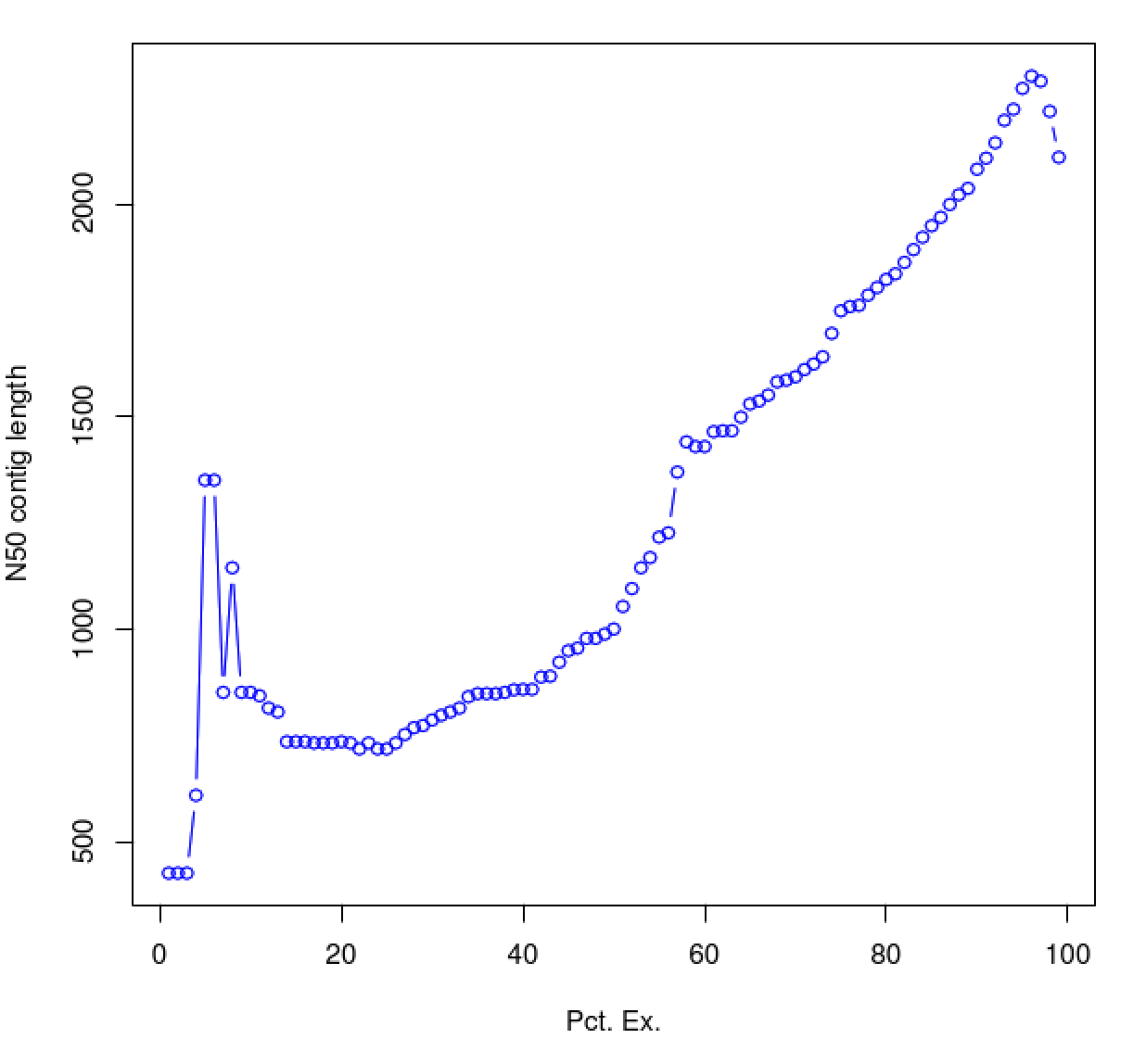
The above table indicates the contig N50 value based on the entire transcriptome assembly (E100), which is a small value (285). By restricting the N50 computation to the set of transcripts representing the top most 65% of expression data, we obtain an N50 value of 420.
Try plotting the ExN50 statistics:
% $TRINITY_HOME/util/misc/plot_ExN50_statistic.Rscript ExN50.stats

% xpdf ExN50.stats.plot.pdf
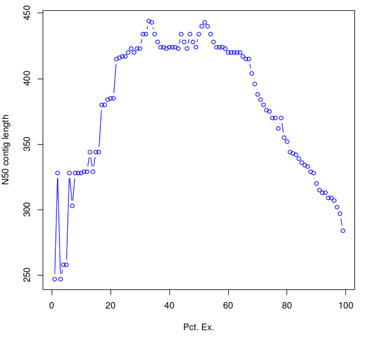
As you can see, the N50 value will tend to peak at a value higher than that computed using the entire data set. With a high quality transcriptome assembly, the N50 value should peak at ~90% of the expression data, which we refer to as the E90N50 value. Reporting the E90N50 contig length and the E90 transcript count are more meaningful than reporting statistics based on the entire set of assembled transcripts. Remember the caveat in assembling this tiny data set. A plot based on a larger set of reads looks like so:
Assembly using 900K PE reads:
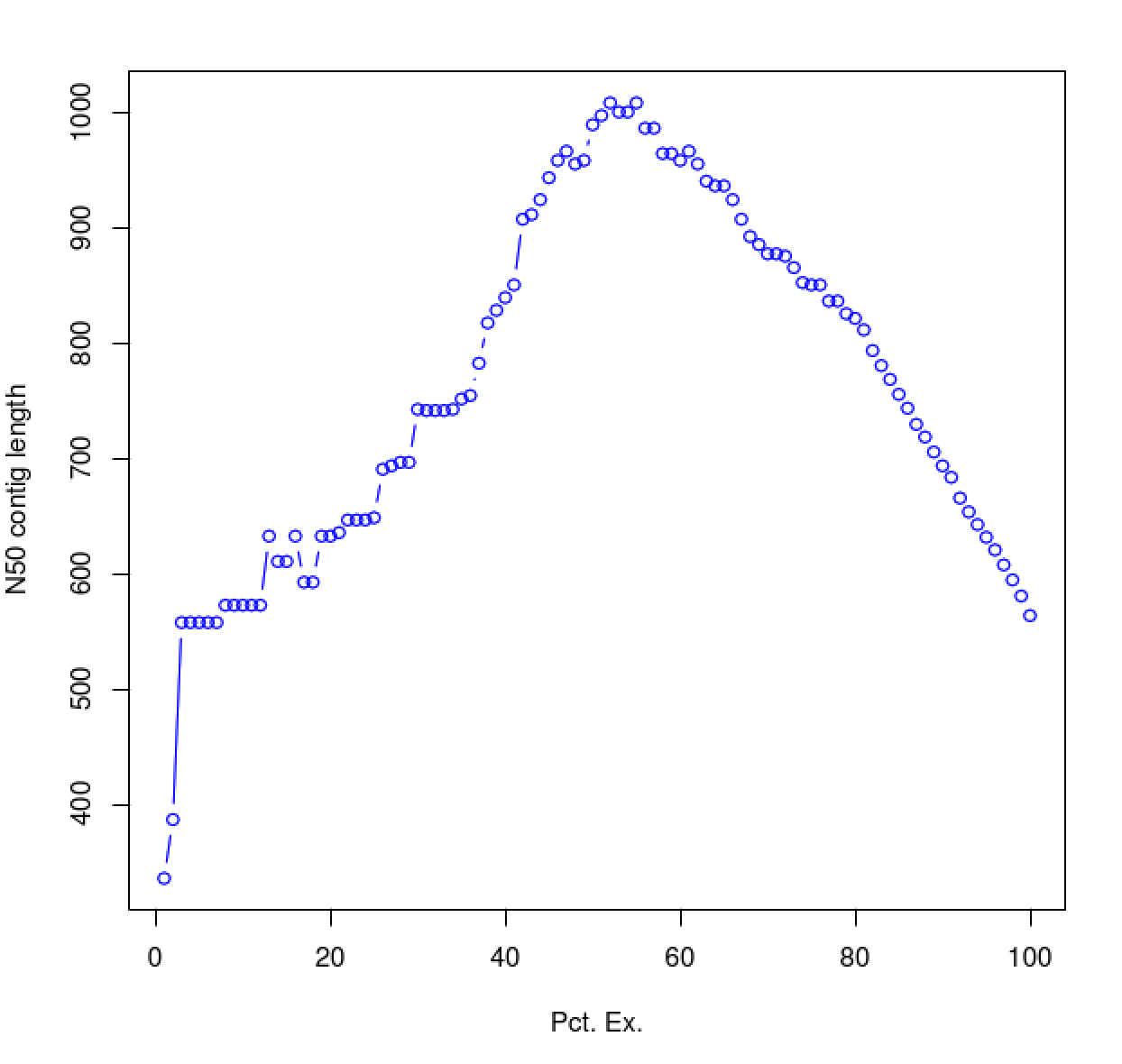
Assembly using 4.5M PE reads:
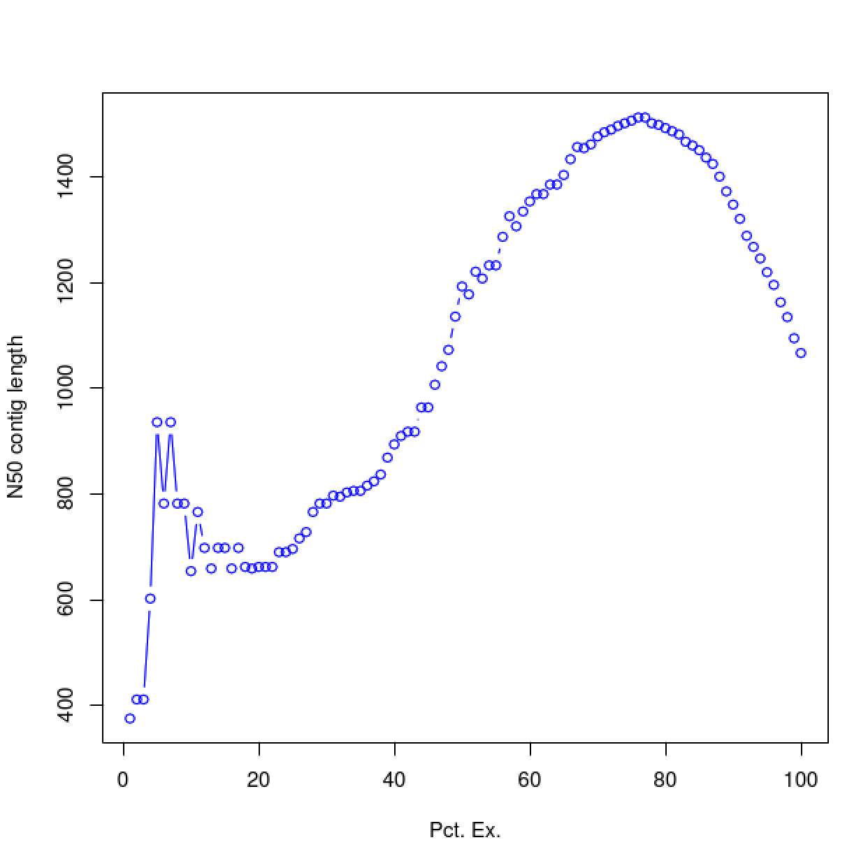
Assembly using 18M PE reads:
You can see that as you sequence deeper, you'll end up with an assembly that has an ExN50 peak that approaches the use of ~90% of the expression data.
Every assembled transcript is only as valid as the reads that support it. If you ever want to examine the read support for one of your favorite transcripts, you could do this using the IGV browser. Earlier, when running RSEM to estimate transcript abundance, we generated bam files containing the reads aligned to the assembled transcripts. Launch IGV on these data like so:
% igv.sh -g trinity_out_dir/Trinity.fasta \
    GSNO_SRR1582648.RSEM/GSNO_SRR1582648.bowtie.csorted.bam,GSNO_SRR1582646.RSEM/GSNO_SRR1582646.bowtie.csorted.bam,GSNO_SRR1582647.RSEM/GSNO_SRR1582647.bowtie.csorted.bam,wt_SRR1582651.RSEM/wt_SRR1582651.bowtie.csorted.bam,wt_SRR1582649.RSEM/wt_SRR1582649.bowtie.csorted.bam,wt_SRR1582650.RSEM/wt_SRR1582650.bowtie.csorted.bam
Note, you could also launch IGV via clicking the icon on the desktop and then manually loading in the various input files via the menu, but that does take some time. Launching it from the command line is rather straightforward and fast.
Take some time to familiarize yourself with IGV. Look at a few transcripts and consider the read support. View the reads as pairs to examine the paired-read linkages.
A plethora of tools are currently available for identifying differentially expressed transcripts based on RNA-Seq data, and of these, edgeR is one of the most popular and most accurate. The edgeR software is part of the R Bioconductor package, and we provide support for using it in the Trinity package.
Having biological replicates for each of your samples is crucial for accurate detection of differentially expressed transcripts. In our data set, we have three biological replicates for each of our conditions, and in general, having three or more replicates for each experimental condition is highly recommended.
Create a samples.txt file containing the contents below (tab-delimited), indicating the name of the condition followed by the name of the biological replicate. Verify the contents of the file using 'cat':
Use your favorite unix text editor (eg. emacs, vim, pico, or nano) to create the file 'samples.txt' containing the tab-delimited contents below. Then verify the contents like so:
% cat samples.txt
.
GSNO	GSNO_SRR1582648
GSNO	GSNO_SRR1582647
GSNO	GSNO_SRR1582646
WT	wt_SRR1582651
WT	wt_SRR1582649
WT	wt_SRR1582650
Here's a trick to verify that you really have tab characters as delimiters:
% cat -te samples.txt
.
GSNO^IGSNO_SRR1582647$
GSNO^IGSNO_SRR1582646$
GSNO^IGSNO_SRR1582648$
WT^Iwt_SRR1582649$
WT^Iwt_SRR1582650$
WT^Iwt_SRR1582651$
There, you should find '^I' at the position of a tab character, and you'll find '$' at the position of a return character. This is invaluable for verifying contents of text files when the formatting has to be very precise. If your view doesn't look exactly as above, then you'll need to re-edit your file and be sure to replace any space characters you see with single tab characters, then re-examine it using the 'cat -te' approach.
The condition name (left column) can be named more or less arbitrarily but should reflect your experimental condition. Importantly, the replicate names (right column) need to match up exactly with the column headers of your RNA-Seq counts matrix.
To detect differentially expressed transcripts, run the Bioconductor package edgeR using our counts matrix:
%  $TRINITY_HOME/Analysis/DifferentialExpression/run_DE_analysis.pl \
      --matrix Trinity_trans.counts.matrix \
      --samples_file samples.txt \
      --method edgeR \
      --output edgeR_trans
Examine the contents of the edgeR_trans/ directory.
% ls -ltr edgeR_trans/
.
-rw-rw-r-- 1 genomics genomics  1051 Jan  9 16:48 Trinity_trans.counts.matrix.GSNO_vs_WT.GSNO.vs.WT.EdgeR.Rscript
-rw-rw-r-- 1 genomics genomics 60902 Jan  9 16:48 Trinity_trans.counts.matrix.GSNO_vs_WT.edgeR.DE_results
-rw-rw-r-- 1 genomics genomics 18537 Jan  9 16:48 Trinity_trans.counts.matrix.GSNO_vs_WT.edgeR.DE_results.MA_n_Volcano.pdf
The files '*.DE_results' contain the output from running EdgeR to identify differentially expressed transcripts in each of the pairwise sample comparisons. Examine the format of one of the files, such as the results from comparing Sp_log to Sp_plat:
% head edgeR_trans/Trinity_trans.counts.matrix.GSNO_vs_WT.edgeR.DE_results | column -t
.
                        logFC              logCPM            PValue                FDR
TRINITY_DN530_c0_g1_i1  8.98959066402695   13.1228060448362  8.32165055033775e-54  5.54221926652494e-51
TRINITY_DN589_c0_g1_i1  4.89839016049723   13.2154341051504  7.57411107973887e-53  2.52217898955304e-50
TRINITY_DN44_c0_g1_i1   2.69777851490106   14.1332252828559  5.23937214153746e-52  1.16314061542132e-49
TRINITY_DN219_c0_g1_i1  5.96230500956404   13.4919132973162  5.11512415417842e-51  8.51668171670708e-49
TRINITY_DN513_c0_g1_i1  5.67480055313841   12.8660937412604  1.54064866426519e-44  2.05214402080123e-42
TRINITY_DN494_c0_g1_i1  8.97722926993194   13.108274725098   3.6100707178792e-44   4.00717849684591e-42
TRINITY_DN365_c0_g1_i1  2.71537635410452   14.0482419858984  8.00431159168039e-41  7.61553074294163e-39
TRINITY_DN415_c0_g1_i1  6.96733684710045   12.875060733337   3.67004658844109e-36  3.05531378487721e-34
TRINITY_DN59_c0_g1_i1   -3.57509574692798  13.1852604213653  3.74452542871713e-30  2.77094881725068e-28
These data include the log fold change (logFC), log counts per million (logCPM), P- value from an exact test, and false discovery rate (FDR).
The EdgeR analysis above generated both MA and Volcano plots based on these data. Examine any of these like so:
% xpdf edgeR_trans/Trinity_trans.counts.matrix.GSNO_vs_WT.edgeR.DE_results.MA_n_Volcano.pdf
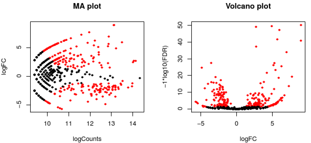
The red data points correspond to all those features that were identified as being significant with an FDR <= 0.05.
Exit the chart viewer to continue.
Trinity facilitates analysis of these data, including scripts for extracting transcripts that are above some statistical significance (FDR threshold) and fold-change in expression, and generating figures such as heatmaps and other useful plots, as described below.
Now let's perform the following operations from within the edgeR_trans/ directory. Enter the edgeR_trans/ dir like so:
% cd edgeR_trans/
Extract those differentially expressed (DE) transcripts that are at least 4-fold differentially expressed at a significance of <= 0.001 in any of the pairwise sample comparisons:
% $TRINITY_HOME/Analysis/DifferentialExpression/analyze_diff_expr.pl \
      --matrix ../Trinity_trans.TMM.EXPR.matrix \
      --samples ../samples.txt \
      -P 1e-3 -C 2
The above generates several output files with a prefix diffExpr.P1e-3_C2', indicating the parameters chosen for filtering, where P (FDR actually) is set to 0.001, and fold change (C) is set to 2^(2) or 4-fold. (These are default parameters for the above script. See script usage before applying to your data).
Included among these files are: ‘diffExpr.P1e-3_C2.matrix’ : the subset of the FPKM matrix corresponding to the DE transcripts identified at this threshold. The number of DE transcripts identified at the specified thresholds can be obtained by examining the number of lines in this file.
% wc -l diffExpr.P1e-3_C2.matrix
.
116 diffExpr.P1e-3_C2.matrix
Note, the number of lines in this file includes the top line with column names, so there are actually 115 DE transcripts at this 4-fold and 1e-3 FDR threshold cutoff.
Also included among these files is a heatmap 'diffExpr.P1e-3_C2.matrix.log2.centered.genes_vs_samples_heatmap.pdf' as shown below, with transcripts clustered along the vertical axis and samples clustered along the horizontal axis.
% xpdf diffExpr.P1e-3_C2.matrix.log2.centered.genes_vs_samples_heatmap.pdf
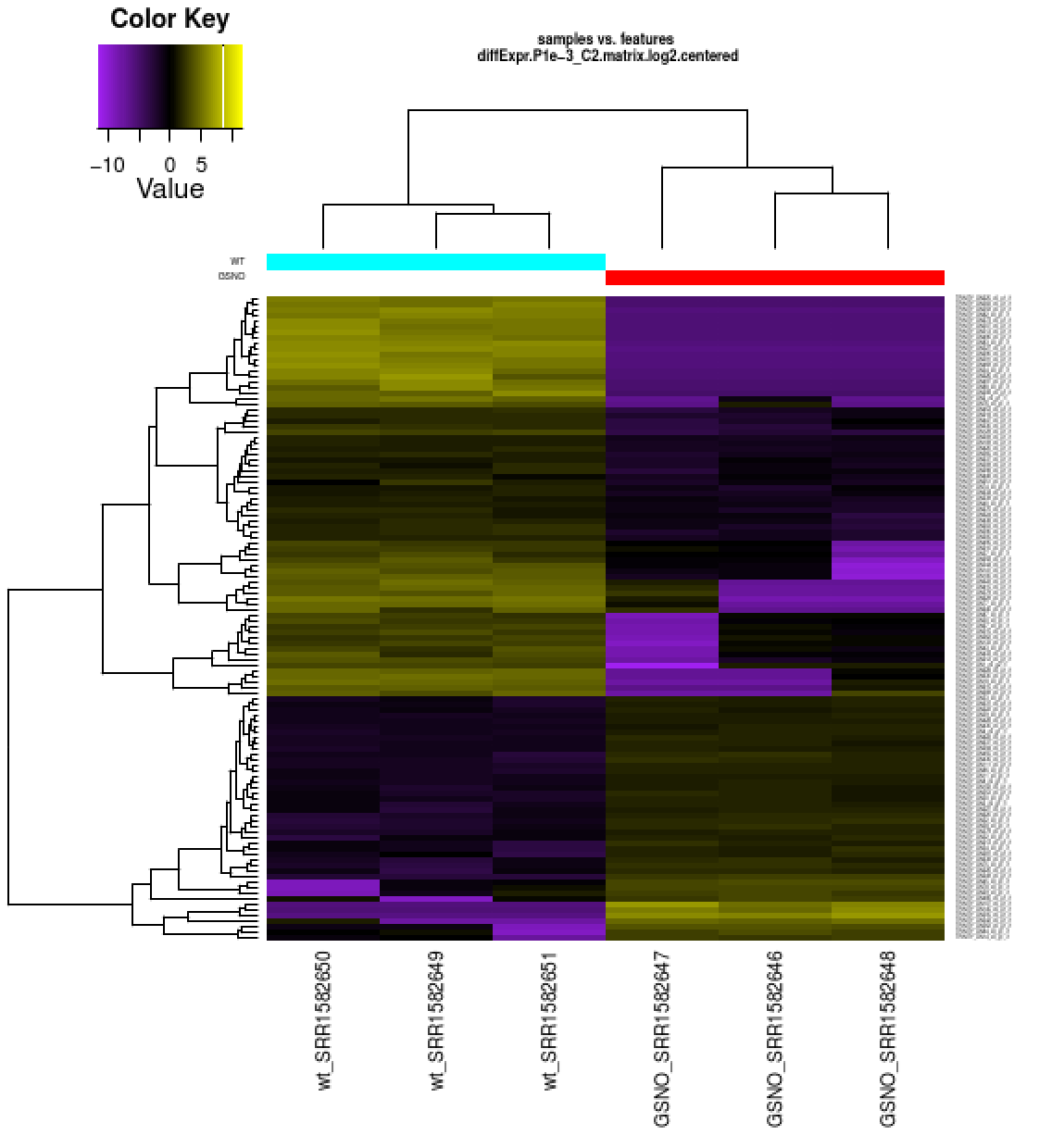
The expression values are plotted in log2 space and mean-centered (mean expression value for each feature is subtracted from each of its expression values in that row), and shows upregulated expression as yellow and downregulated expression as purple.
Exit the PDF viewer to continue.
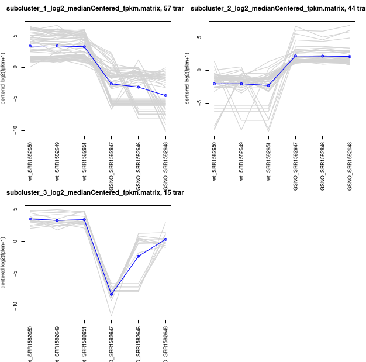
Extract clusters of transcripts with similar expression profiles by cutting the transcript cluster dendrogram at a given percent of its height (ex. 60%), like so:
% $TRINITY_HOME/Analysis/DifferentialExpression/define_clusters_by_cutting_tree.pl \
       --Ptree 60 -R diffExpr.P1e-3_C2.matrix.RData
This creates a directory containing the individual transcript clusters, including a pdf file that summarizes expression values for each cluster according to individual charts:
% xpdf diffExpr.P1e-3_C2.matrix.RData.clusters_fixed_P_60/my_cluster_plots.pdf
You can do all the same analyses as you did above at the gene level. For now, let's just rerun the DE detection step, since we'll need the results later on for use with TrinotateWeb. Also, it doesn't help us to study the 'gene' level data with this tiny data set (yet another disclaimer) given that all our transcripts = genes, since we didn't find any alternative splicing variants. With typical data sets, you will have alterantively spliced isoforms identified, and performing DE analysis at the gene level should provide more power for detection than at the isoform level. For more info about this, I encourage you to read this paper.
Before running the gene-level DE analysis, be sure to back out of the current edgeR_trans/ directory like so:
% cd ../
Be sure you're in your base working directory:
% pwd
.
/home/genomics/workshop_data/transcriptomics/KrumlovTrinityWorkshopJan2016
Now, run the DE analysis at the gene level like so:
%  $TRINITY_HOME/Analysis/DifferentialExpression/run_DE_analysis.pl \
      --matrix Trinity_genes.counts.matrix \
      --samples_file samples.txt \
      --method edgeR \
      --output edgeR_gene
You'll now notice that the edgeR_gene/ directory exists and is populated with similar files.
% ls -ltr edgeR_gene/
Let's move on and make use of those outputs later. With your own data, however, you would normally run the same set of operations as you did above for the transcript-level DE analyses.
Now we have a bunch of transcript sequences and have identified some subset of them that appear to be biologically interesting in that they're differentially expressed between our two conditions - but we don't really know what they are or what biological functions they might represent. We can explore their potential functions by functionally annotating them using our Trinotate software and analysis protocol. To learn more about Trinotate, you can visit the Trinotate website.
Again, let's make sure that we're back in our primary working directory called 'KrumlovTrinityWorkshopJan2016':
% pwd
.
/home/genomics/workshop_data/transcriptomics/KrumlovTrinityWorkshopJan2016
If you're not in the above directory, then relocate yourself to it.
Now, create a Trinotate/ directory and relocate to it. We'll use this as our Trinotate computation workspace.
% mkdir Trinotate

% cd Trinotate
Below, we're going to run a number of different tools to capture information about our transcript sequences.
TransDecoder is a tool we built to identify likely coding regions within transcript sequences. It identifies long open reading frames (ORFs) within transcripts and scores them according to their sequence composition. Those ORFs that encode sequences with compositional properties (codon frequencies) consistent with coding transcripts are reported.
Running TransDecoder is a two-step process. First run the TransDecoder step that identifies all long ORFs.
% $TRANSDECODER_HOME/TransDecoder.LongOrfs -t ../trinity_out_dir/Trinity.fasta
Now, run the step that predicts which ORFs are likely to be coding.
% $TRANSDECODER_HOME/TransDecoder.Predict -t ../trinity_out_dir/Trinity.fasta
You'll now find a number of output files containing 'transdecoder' in their name:
% ls -1 |grep transdecoder
.
Trinity.fasta.transdecoder.bed
Trinity.fasta.transdecoder.cds
Trinity.fasta.transdecoder.gff3
Trinity.fasta.transdecoder.mRNA
Trinity.fasta.transdecoder.pep
Trinity.fasta.transdecoder_dir/
The file we care about the most here is the 'Trinity.fasta.transdecoder.pep' file, which contains the protein sequences corresponding to the predicted coding regions within the transcripts.
Go ahead and take a look at this file:
% less Trinity.fasta.transdecoder.pep
.
>TRINITY_DN102_c0_g1_i1|m.9 TRINITY_DN102_c0_g1_i1|g.9  ORF TRINITY_DN102_c0_g1_i1|g.9 \
    TRINITY_DN102_c0_g1_i1|m.9 type:complete len:185 (+) TRINITY_DN102_c0_g1_i1:23-577(+)
MARYGATSTNPAKSASARGSYLRVSFKNTRETAQAINGWELTKAQKYLDQVLEHQRAIPF
RRYNSSIGRTAQGKEFGVTKARWPAKSVKFIQGLLQNAAANAEAKGLDATKLYVSHIQVN
HAPKQRRRTYRAHGRINKYESSPSHIELVVTEKEEAVAKAAEKKLVRLSSRQRGRIASQK
RITA*
>TRINITY_DN106_c0_g1_i1|m.3 TRINITY_DN106_c0_g1_i1|g.3  ORF TRINITY_DN106_c0_g1_i1|g.3 \
    TRINITY_DN106_c0_g1_i1|m.3 type:5prime_partial len:149 (-) TRINITY_DN106_c0_g1_i1:38-484(-)
TNDTNESNTRTMSGNGAQGTKFRISLGLPTGAIMNCADNSGARNLYIMAVKGSGSRLNRL
PAASLGDMVMATVKKGKPELRKKVMPAIVVRQSKAWRRKDGVYLYFEDNAGVIANPKGEM
KGSAITGPVGKECADLWPRVASNSGVVV*
>TRINITY_DN109_c0_g1_i1|m.14 TRINITY_DN109_c0_g1_i1|g.14  ORF TRINITY_DN109_c0_g1_i1|g.14 \
    TRINITY_DN109_c0_g1_i1|m.14 type:internal len:102 (+) TRINITY_DN109_c0_g1_i1:2-304(+)
AKVTDLRDAMFAGEHINFTEDRAVYHVALRNRANKPMKVDGVDVAPEVDAVLQHMKEFSE
QVRSGEWKGYTGKKITDVVNIGIGGSDLGPVMVTEALKHYA
>TRINITY_DN113_c0_g1_i1|m.16 TRINITY_DN113_c0_g1_i1|g.16  ORF TRINITY_DN113_c0_g1_i1|g.16 \
    TRINITY_DN113_c0_g1_i1|m.16 type:3prime_partial len:123 (-) TRINITY_DN113_c0_g1_i1:2-367(-)
MSDSVTIRTRKVITNPLLARKQFVVDVLHPNRANVSKDELREKLAEAYKAEKDAVSVFGF
RTQFGGGKSTGFGLVYNSVADAKKFEPTYRLVRYGLAEKVEKASRQQRKQKKNRDKKIFG
TG
Type 'q' to exit the 'less' viewer.
There are a few items to take notice of in the above peptide file. The header lines includes the protein identifier composed of the original transcripts along with '|m.(number)'. The 'type' attribute indicates whether the protein is 'complete', containing a start and a stop codon; '5prime_partial', meaning it's missing a start codon and presumably part of the N-terminus; '3prime_partial', meaning it's missing the stop codon and presumably part of the C-terminus; or 'internal', meaning it's both 5prime-partial and 3prime-partial. You'll also see an indicator (+) or (-) to indicate which strand the coding region is found on, along with the coordinates of the ORF in that transcript sequence.
This .pep file will be used for various sequence homology and other bioinformatics analyses below.
Earlier, we ran blastx against our mini SWISSPROT datbase to identify likely full-length transcripts. Let's run blastx again to capture likely homolog information, and we'll lower our E-value threshold to 1e-5 to be less stringent than earlier.
% blastx -db ../data/mini_sprot.pep \
         -query ../trinity_out_dir/Trinity.fasta -num_threads 2 \
         -max_target_seqs 1 -outfmt 6 -evalue 1e-5 \
          > swissprot.blastx.outfmt6
Now, let's look for sequence homologies by just searching our predicted protein sequences rather than using the entire transcript as a target:
% blastp -query Trinity.fasta.transdecoder.pep \
         -db ../data/mini_sprot.pep -num_threads 2 \
         -max_target_seqs 1 -outfmt 6 -evalue 1e-5 \
          > swissprot.blastp.outfmt6
Using our predicted protein sequences, let's also run a HMMER search against the Pfam database, and identify conserved domains that might be indicative or suggestive of function:
% hmmscan --cpu 2 --domtblout TrinotatePFAM.out \
          ../../trinnotate_databases/Pfam-A.hmm \
          Trinity.fasta.transdecoder.pep
Note, hmmscan might take a few minutes to run.
The signalP and tmhmm software tools are very useful for predicting signal peptides (secretion signals) and transmembrane domains, respectively.
To predict signal peptides, run signalP like so:
% signalp -f short -n signalp.out Trinity.fasta.transdecoder.pep
Take a look at the output file:
% less signalp.out
.
##gff-version 2
##sequence-name source  feature start   end     score   N/A ?
## -----------------------------------------------------------
TRINITY_DN19_c0_g1_i1|m.141     SignalP-4.0     SIGNAL  1       18      0.553   .       .       YES
TRINITY_DN33_c0_g1_i1|m.174     SignalP-4.0     SIGNAL  1       19      0.631   .       .       YES
....
How many of your proteins are predicted to encode signal peptides?
To predict transmembrane domain predictions, run tmhmm like so:
% tmhmm --short < Trinity.fasta.transdecoder.pep > tmhmm.out
Take a look at the output:
% less tmhmm.out
.
TRINITY_DN56_c0_g1_i1|m.126     len=303 ExpAA=126.72    First60=16.21   PredHel=6       Topology=o44-66i100-119o129-148i155-177o187-209i222-241o
TRINITY_DN56_c0_g2_i1|m.127     len=262 ExpAA=126.02    First60=23.86   PredHel=6       Topology=o5-24i59-78o88-107i114-136o146-168i181-200o
Those entries that have results contain output like so 'Topology=o5-24i59-78o88-107i114-136o146-168i181-200o' are the predicted transmembrane proteins. The number of helices in the transmembrane domain is listed under PredHel=(number) and the topology indicates the region within the protein sequence that spans the membrane from (i) inside to (o) outside the cell.
Generating a Trinotate annotation report involves first loading all of our bioinformatics computational results into a Trinotate SQLite database. The Trinotate software provides a boilerplate SQLite database called 'Trinotate.sqlite' that comes pre-populated with a lot of generic data about SWISSPROT records and Pfam domains (and is a pretty large file consuming several GB). Below, we'll populate this database with all of our bioinformatics computes and our expression data. You'll find your 'Trinotate.sqlite' database in your base working directory for this workshop (ie. '/..../KrumlovTrinityWorkshopJan2016/Trinotate.sqlite').
As a sanity check, be sure you're currently located in your 'Trinotate/' working directory.
% pwd
.
/home/genomics/workshop_data/transcriptomics/KrumlovTrinityWorkshopJan2016/Trinotate
Load your Trinotate.sqlite database with your Trinity transcripts and predicted protein sequences:
%  $TRINOTATE_HOME/Trinotate ../Trinotate.sqlite init \
     --gene_trans_map ../trinity_out_dir/Trinity.fasta.gene_trans_map \
     --transcript_fasta ../trinity_out_dir/Trinity.fasta \
     --transdecoder_pep Trinity.fasta.transdecoder.pep
Load in the various outputs generated earlier:
%  $TRINOTATE_HOME/Trinotate ../Trinotate.sqlite \
       LOAD_swissprot_blastx swissprot.blastx.outfmt6

%  $TRINOTATE_HOME/Trinotate ../Trinotate.sqlite \
       LOAD_swissprot_blastp swissprot.blastp.outfmt6

%  $TRINOTATE_HOME/Trinotate ../Trinotate.sqlite LOAD_pfam TrinotatePFAM.out

%  $TRINOTATE_HOME/Trinotate ../Trinotate.sqlite LOAD_tmhmm tmhmm.out

%  $TRINOTATE_HOME/Trinotate ../Trinotate.sqlite LOAD_signalp signalp.out
% $TRINOTATE_HOME/Trinotate ../Trinotate.sqlite report > Trinotate.xls
View the report
% less Trinotate.xls
.
#gene_id        transcript_id   sprot_Top_BLASTX_hit    TrEMBL_Top_BLASTX_hit   RNAMMER prot_id prot_coords     sprot_Top_BLASTP_hit    TrEMBL_Top_BLASTP_hit   Pfam    SignalP TmHMM   eggnog  gene_ontology_blast     gene_ontology_pfam      transcript      peptide
TRINITY_DN144_c0_g1     TRINITY_DN144_c0_g1_i1  PUT4_YEAST^PUT4_YEAST^Q:1-198,H:425-490^74.24%ID^E:4e-29^RecName: Full=Proline-specific permease;^Eukaryota; Fungi; Dikarya; Ascomycota; Saccharomycotina; Saccharomycetes; Saccharomycetales; Saccharomycetaceae; Saccharomyces        .       .       .       .
   .       .       .       .       .       COG0833^permease        GO:0016021^cellular_component^integral component of membrane`GO:0005886^cellular_component^plasma membrane`GO:0015193^molecular_function^L-proline transmembrane transporter activity`GO:0015175^molecular_function^neutral amino acid transmembrane transporter activity`GO:0015812^biological_process^gamma-aminobutyric acid transport`GO:0015804^biological_process^neutral amino acid transport`GO:0035524^biological_process^proline transmembrane transport`GO:0015824^biological_process^proline transport      .       .       .
TRINITY_DN179_c0_g1     TRINITY_DN179_c0_g1_i1  ASNS1_YEAST^ASNS1_YEAST^Q:1-168,H:158-213^82.14%ID^E:5e-30^RecName: Full=Asparagine synthetase [glutamine-hydrolyzing] 1;^Eukaryota; Fungi; Dikarya; Ascomycota; Saccharomycotina; Saccharomycetes; Saccharomycetales; Saccharomycetaceae; Saccharomyces        .
   .       .       .       .       .       .       .       .       COG0367^asparagine synthetase   GO:0004066^molecular_function^asparagine synthase (glutamine-hydrolyzing) activity`GO:0005524^molecular_function^ATP binding`GO:0006529^biological_process^asparagine biosynthetic process`GO:0006541^biological_process^glutamine metabolic process`GO:0070981^biological_process^L-asparagine biosynthetic process    .       .       .
TRINITY_DN159_c0_g1     TRINITY_DN159_c0_g1_i1  ENO2_CANGA^ENO2_CANGA^Q:2-523,H:128-301^100%ID^E:4e-126^RecName: Full=Enolase 2;^Eukaryota; Fungi; Dikarya; Ascomycota; Saccharomycotina; Saccharomycetes; Saccharomycetales; Saccharomycetaceae; Nakaseomyces; Nakaseomyces/Candida clade      .       .       TRINITY_DN159_c0_g1_i1|m.1      2-523[+]        ENO2_CANGA^ENO2_CANGA^Q:1-174,H:128-301^100%ID^E:3e-126^RecName: Full=Enolase 2;^Eukaryota; Fungi; Dikarya; Ascomycota; Saccharomycotina; Saccharomycetes; Saccharomycetales; Saccharomycetaceae; Nakaseomyces; Nakaseomyces/Candida clade      .       PF00113.17^Enolase_C^Enolase, C-terminal TIM barrel domain^18-174^E:9.2e-79     .       .       .       GO:0005829^cellular_component^cytosol`GO:0000015^cellular_component^phosphopyruvate hydratase complex`GO:0000287^molecular_function^magnesium ion binding`GO:0004634^molecular_function^phosphopyruvate hydratase activity`GO:0006096^biological_process^glycolytic process     GO:0000287^molecular_function^magnesium ion binding`GO:0004634^molecular_function^phosphopyruvate hydratase activity`GO:0006096^biological_process^glycolytic process`GO:0000015^cellular_component^phosphopyruvate hydratase complex   .       .
...
The above file can be very large. It's often useful to load it into a spreadsheet software tools such as MS-Excel. If you have a transcript identifier of interest, you can always just 'grep' to pull out the annotation for that transcript from this report. We'll use TrinotateWeb to interactively explore these data in a web browser below.
Let's use the annotation attributes for the transcripts here as 'names' for the transcripts in the Trinotate database. This will be useful later when using the TrinotateWeb framework.
%  $TRINOTATE_HOME/util/annotation_importer/import_transcript_names.pl \
      ../Trinotate.sqlite Trinotate.xls
Nothing exciting to see in running the above command, but know that it's helpful for later on.
Notice that the report above contains Gene Ontology identifiers mapped to transcripts. These are derived from SWISSPROT records of matching proteins as well as assigned according to Pfam domain content. The Gene Ontology structured classifications will allow us to explore whether we have statistically significant functional enrichment based on gene sets - such as for those genes that were identified to be differentially expressed.
Generate a listing of all GO identifiers assigned to each transcript like so:
% $TRINOTATE_HOME/util/extract_GO_assignments_from_Trinotate_xls.pl \
       --Trinotate_xls Trinotate.xls -T -I > Trinotate.xls.gene_ontology
If you see warning messages 'cannot parse parent info', simply ignore them.
and take a look at the output file:
% less Trinotate.xls.gene_ontology
.
TRINITY_DN101_c0_g1_i1  GO:0003674,GO:0003824,GO:0005488,GO:0005506,GO:0005575,GO:0005759,GO:0005829,GO:0006810,GO:0006950,GO:0006979,GO:0008150,GO:0008941,GO:0009636,GO:0009987,GO:0015669,GO:0015671,GO:0016491,GO:0016661,GO:0016662,GO:0016705,GO:0016708,GO:0016966,GO:0019825,GO:0020037,GO:0031974,GO:0033554,GO:0034599,GO:0042221,GO:0043167,GO:0043169,GO:0043233,GO:0044422,GO:0044424,GO:0044429,GO:0044444,GO:0044446,GO:0044464,GO:0044699,GO:0044765,GO:0046872,GO:0046906,GO:0046914,GO:0050896,GO:0051179,GO:0051213,GO:0051234,GO:0051716,GO:0070013,GO:0070887,GO:0097159,GO:1901363,GO:1902578
TRINITY_DN102_c0_g1_i1  GO:0002181,GO:0003674,GO:0003735,GO:0005198,GO:0005575,GO:0005840,GO:0006412,GO:0008150,GO:0008152,GO:0009058,GO:0009059,GO:0009987,GO:0015934,GO:0019538,GO:0022625,GO:0030529,GO:0032991,GO:0034645,GO:0043170,GO:0043226,GO:0043228,GO:0043229,GO:0043232,GO:0044237,GO:0044238,GO:0044249,GO:0044260,GO:0044267,GO:0044391,GO:0044422,GO:0044424,GO:0044444,GO:0044445,GO:0044446,GO:0044464,GO:0071704,GO:1901576
TRINITY_DN103_c0_g1_i1  GO:0003674,GO:0003824,GO:0004130,GO:0004601,GO:0005488,GO:0005575,GO:0005759,GO:0005829,GO:0006950,GO:0006979,GO:0008150,GO:0016209,GO:0016491,GO:0016684,GO:0020037,GO:0031974,GO:0043167,GO:0043169,GO:0043233,GO:0044422,GO:0044424,GO:0044429,GO:0044444,GO:0044446,GO:0044464,GO:0046872,GO:0046906,GO:0050896,GO:0070013,GO:0097159,GO:1901363
...
Now that we have our list of transcript-to-GO assignment mappings, let's go back to the edgeR directory and explore functional enrichments of our DE transcripts:
% cd ../edgeR_trans
We'll use the GOseq software to test for GO enrichment. One of the key merits of GOseq is that it takes into account biases in transcript feature lengths according to functional categories (some functional categories have many long or short proteins, which biases their representation as detected in DE data). Generate a file containing the lengths of each of our assembled transcripts like so:
% $TRINITY_HOME/util/misc/fasta_seq_length.pl \
     ../trinity_out_dir/Trinity.fasta > Trinity.seqLengths
Take a glance at the file we just generated:
% less Trinity.seqLengths
.
fasta_entry             length
TRINITY_DN144_c0_g1_i1  199
TRINITY_DN179_c0_g1_i1  169
TRINITY_DN159_c0_g1_i1  524
TRINITY_DN153_c0_g1_i1  182
TRINITY_DN130_c0_g1_i1  254
Now, run GOseq on our subset of transcripts that were identified as significantly DE given our earlier chosen thresholds. We'll start with the subset of transcripts that were identified as significantly upregulated under the GSNO treatment:
%  $TRINITY_HOME/Analysis/DifferentialExpression/run_GOseq.pl \
      --genes_single_factor Trinity_trans.counts.matrix.GSNO_vs_WT.edgeR.DE_results.P1e-3_C2.GSNO-UP.subset \
      --GO_assignments ../Trinotate/Trinotate.xls.gene_ontology \
      --lengths Trinity.seqLengths
This will generate two output files, one containing GO categories enriched among that set of DE transcripts (.GSNO-UP.subset.GOseq.enriched), and another containing GO categores that are depleted (.GSNO-UP.subset.GOseq.depleted).
Examine the contents of these files using 'less'.
Note, the small number of reads we are using for the assembly and DE analysis is going to hinder our sensitivity for detection of DE transcripts and this will funnel into a lack of sensitivity in picking up functional category enrichments. We do identify functional category enrichments here, but the most informative findings would require assembling the original millions of RNA-Seq reads to find them.
You can run the same GOseq functional enrichment analysis on those transcripts that were found significantly upregulated under the rich media growth conditions.
%  $TRINITY_HOME/Analysis/DifferentialExpression/run_GOseq.pl \
      --genes_single_factor Trinity_trans.counts.matrix.GSNO_vs_WT.edgeR.DE_results.P1e-3_C2.WT-UP.subset \
      --GO_assignments ../Trinotate/Trinotate.xls.gene_ontology \
      --lengths Trinity.seqLengths
See which files were just generated as a result:
% ls -ltr
and view each to see if there's anything interesting. Remember the caveat mentioned above about not being well powered in having used our small example set of reads.
Earlier, we generated large sets of tab-delimited files containg lots of data - annotations for transcripts, matrices of expression values, lists of differentially expressed transcripts, etc. We also generated a number of plots in PDF format. These are all useful, but they're not interactive and it's often difficult and cumbersome to extract information of interest during a study. We're developing TrinotateWeb as a web-based interactive system to solve some of these challenges. TrinotateWeb provides heatmaps and various plots of expression data, and includes search functions to quickly access information of interest. Below, we will populate some of the additional information that we need into our Trinotate database, and then run TrinotateWeb and start exploring our data in a web browser.
Let's change our working directory back to the Trinotate/ workspace:
% cd ../Trinotate
Now, load in the transcript expression data stored in the matrices we built earlier:
%  $TRINOTATE_HOME/util/transcript_expression/import_expression_and_DE_results.pl \
        --sqlite ../Trinotate.sqlite \
        --transcript_mode \
        --samples_file ../samples.txt \
        --count_matrix ../Trinity_trans.counts.matrix \
        --fpkm_matrix ../Trinity_trans.TMM.EXPR.matrix
Import the DE results from our edgeR_trans/ directory:
%  $TRINOTATE_HOME/util/transcript_expression/import_expression_and_DE_results.pl \
       --sqlite ../Trinotate.sqlite \
       --transcript_mode \
       --samples_file ../samples.txt \
       --DE_dir ../edgeR_trans
and Import the clusters of transcripts we extracted earlier based on having similar expression profiles across samples:
%  $TRINOTATE_HOME/util/transcript_expression/import_transcript_clusters.pl \
       --sqlite ../Trinotate.sqlite \
       --group_name DE_all_vs_all \
       --analysis_name diffExpr.P1e-3_C2.matrix.RData.clusters_fixed_P_60 \
        ../edgeR/diffExpr.P1e-3_C2.matrix.RData.clusters_fixed_P_60/*matrix
And now we'll do the same for our gene-level expression and DE results:
%  $TRINOTATE_HOME/util/transcript_expression/import_expression_and_DE_results.pl \
        --sqlite ../Trinotate.sqlite \
        --component_mode \
        --samples_file ../samples.txt \
        --count_matrix ../Trinity_genes.counts.matrix \
        --fpkm_matrix ../Trinity_genes.TMM.EXPR.matrix


%  $TRINOTATE_HOME/util/transcript_expression/import_expression_and_DE_results.pl \
       --sqlite ../Trinotate.sqlite \
       --component_mode \
       --samples_file ../samples.txt \
       --DE_dir ../edgeR_gene
Note, in the above gene-loading commands, the term 'component' is used. 'Component' is just another word for 'gene' in the realm of Trinty.
At this point, the Trinotate database should be fully populated and ready to be used by TrinotateWeb.
TrinotateWeb is web-based software and runs locally on the same hardware we've been running all our computes (as opposed to your typical websites that you visit regularly, such as facebook). Launch the mini webserver that drives the TrinotateWeb software like so:
% $TRINOTATE_HOME/run_TrinotateWebserver.pl 3000
Now, visit the following URL in Google Chrome: http://localhost:3000/cgi-bin/index.cgi
You should see a web form like so:
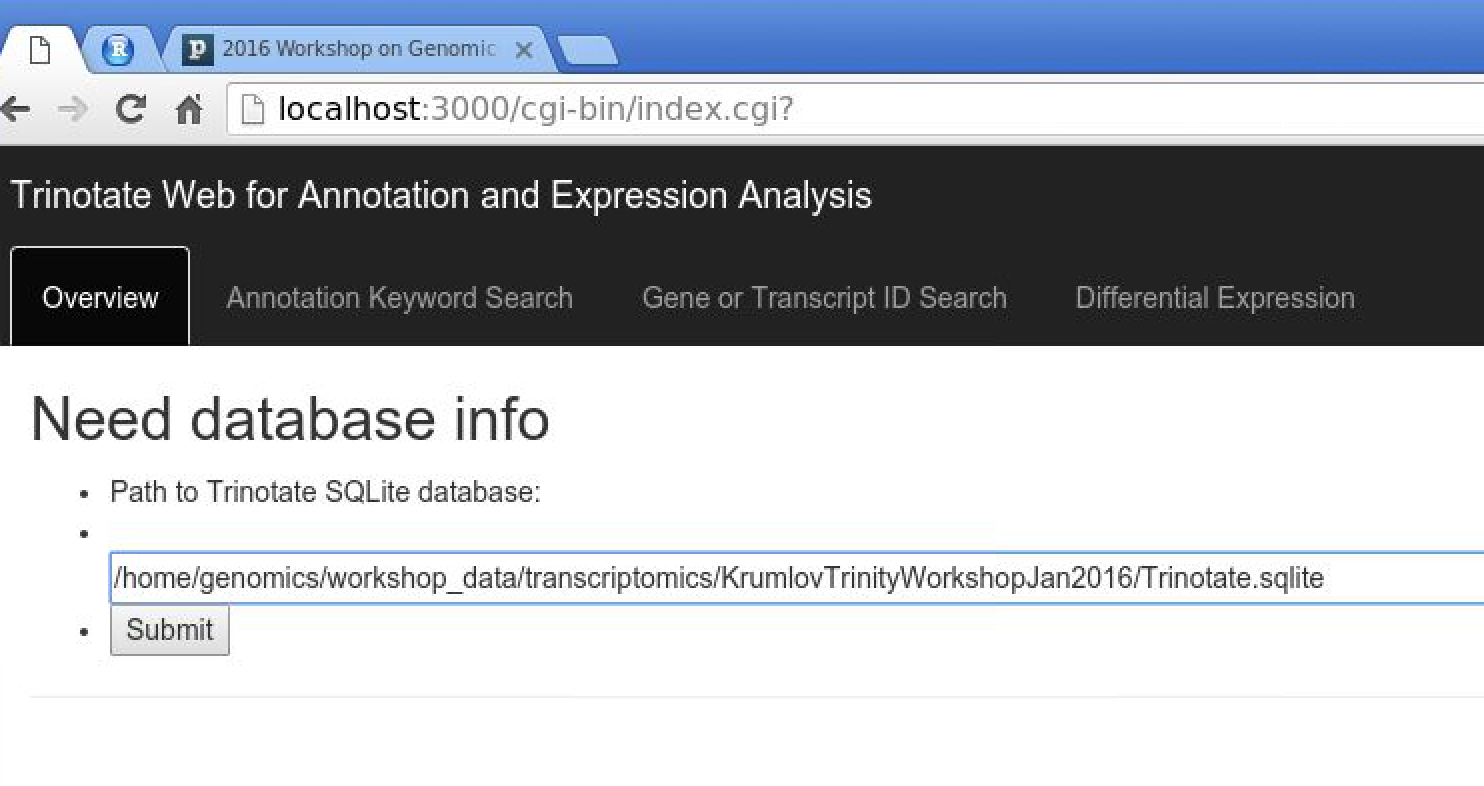
In the text box, put the path to your Trinotate.sqlite database, as shown above ("/home/genomics/workshop_data/transcriptomics/KrumlovTrinityWorkshopJan2016/Trinotate.sqlite"). Click 'Submit'.
You should now have TrinotateWeb running and serving the content in your Trinotate database:
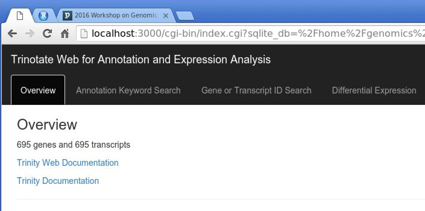
Take some time to click the various tabs and explore what's available.
eg. Under 'Annotation Keyword Search', search for 'transporter'
eg. Under 'Differential Expression', examine your earlier-defined transcript clusters. Also, launch MA or Volcano plots to explore the DE data.
We will explore TrinotateWeb functionality together as a group.
If you've gotten this far, hurray!!! Congratulations!!! You've now experienced the full tour of Trinity and TrinotateWeb. Visit our web documentation at http://trinityrnaseq.github.io, and join our Google group to become part of the ever-growing Trinity user community.