4.6MBAR.md

MBAR Estimator

1. Theory

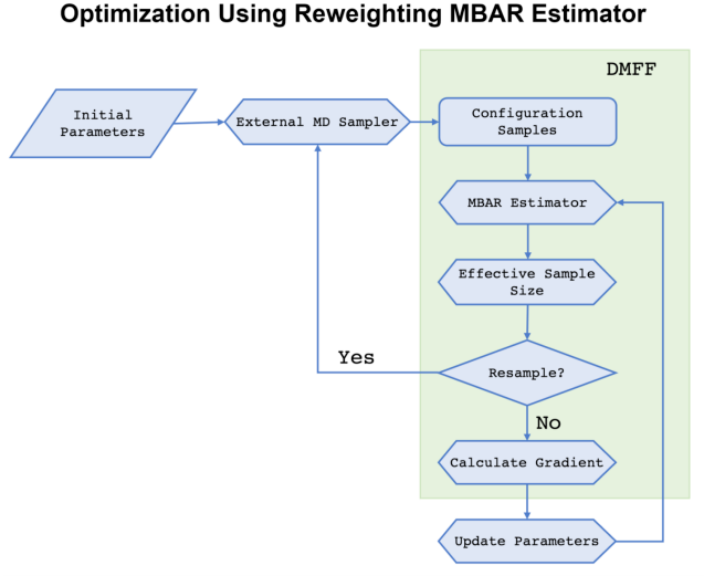
In molecular dynamics (MD) simulations, the deep computational graph spanning the entire trajectory incurs significant temporal and computational costs. This limitation can be circumvented through trajectory reweighting schemes. In DMFF, the reweighting algorithm is incorporated into the MBAR method, extending the differentiable estimators for average properties and free energy. Although differentiable estimation of dynamic properties remains a challenge, introducing the reweighted MBAR estimator has largely eased the fitting of thermodynamic properties.

In the MBAR theory, it is assumed that there are K ensembles defined by (effective) potential energies

$$\tag{1} u_{i}(x)\ (i=1,2,3,……,K)$$

For each ensemble, the Boltzmann weight, partition function, and probability function are defined as:

$$\tag{2} \begin{align} w_i &= \exp(-\beta_i u_i(x)) \\\ c_i &= \int dx \cdot w_i(x) \\\ p_i(x) &= \frac{w_i(x)}{c_i} \end{align}$$

For each ensemble $i$, select $N_{i}$ configurations, represented by { ${x_{in}}$ } $n=1,2,3,……,N_i$ , and the total number of configurations across ensembles is represented by { ${x_{n}}$ } ( $n=1,2,3,……,N$ ), where N is:

$$\tag{3} N = \sum_{i=1}^{K} N_i$$

Within the context of MBAR, for any ensemble K, the weighted average of the observable is defined as:

$$\tag{4} \hat{c}_i = \sum_{n=1}^{N} w_{i}(x_n) \cdot \left(\sum_{k=1}^{K} N_{k} \hat{c}_k^{-1} w_{k}(x_n)\right)^{-1}$$

To compute the average of a physical quantity $A$ in ensemble $i$, one can utilize the above values to define a virtual ensemble $j$ , with its corresponding Boltzmann weight and partition function:

$$\tag{5} \begin{align} w_j &= w_i(x)A(x) \\\ c_i &= \int dx \cdot w_j(x) \end{align}$$

Thus, the ensemble average of A is:

$$\tag{6} \langle A \rangle_i = \frac{\hat{c}_j}{\hat{c}_i} = \frac{\int dx \cdot w_i(x)A(x)}{\int dx \cdot w_i(x)}$$

Thus, the MBAR theory provides a method to estimate the ensemble averages using multiple samples from different ensembles.

In the MBAR framework, $\hat{c}_i$ in Eqn (4) needs to be solved iteratively; however, the differentiable reweighting algorithm can simplify this estimation process. During the gradient descent parameter optimization, the parameters undergo only small changes in each training cycle. This allows for the usage of samples from the previous cycles to evaluate the target ensemble that is being optimized. So resampling is not necessary until the target ensemble deviates significantly from the sampling ensemble. This reduces the time and computational cost of the optimization considerably.

In the reweighted MBAR estimator, we define two types of ensembles: the sampling ensemble, from which all samples are extracted (labeled as $m=1, 2, 3, …, M$ ), and the target ensemble, which needs optimization (labeled as $p, q$, corresponding to the indices $i, j$ in Eqn (6)). The sampling ensemble is updated only when necessary and does not need to be differentiable. Its data can be generated by external samplers like OpenMM. Hence, $\hat{c}_i$ can be transformed into:

$$\tag{7} \hat{c}_p = \sum_{n=1}^{N} w_{p}(x_n) \left( \sum_{m=1}^{M} N_{m} \hat{c}_m^{-1} w_{m}(x_n) \right)^{-1}$$

When resample happens, Eqn. (4) is solved iteratively using standard MBAR to update $\hat{c}_m$, which is stored and used to evaluate $\hat{c}_p$ until the next resampling. Subsequently, during the parameter optimization process, Eqn (7) is employed to compute $\hat{c}_p$, serving as a differentiable estimator.

Below, we illustrate the workflow of how to use MBAR Estimator in DMFF through a case study.

If all sampling ensembles are defined as a single ensemble $w_{0}(x)$, and the target ensemble is defined as $w_{p}(x)$, and for physical quantity A, we have:

$$\tag{8} w_q(x) = w_p(x) A(x)$$

and define:

$$\tag{9} \Delta u_{p_0} = u_p(x) - u_0(x)$$

then:

$$\tag{10} \langle A \rangle_p = \frac{\hat{c}_q}{\hat{c}_p} = \left(\sum_{n=1}^{N} A(x_n) \exp(-\beta \Delta u_{p_0}(x_n))\right) \cdot \left(\sum_{n=1}^{N} \exp(-\beta \Delta u_{p_0}(x_n))\right)^{-1}$$

Refers to equations above, this equation indicates that the trajectory reweighting algorithm is a special case of the reweighted MBAR estimator.

In DMFF, when calculating the average of the physical quantity A, the formula is expressed as:

$$\tag{11} \langle A \rangle_p = \sum_{n=1}^{N} W_n A(x_n)$$

where

$$\tag{12} \Delta U_{mp} = U_m(x_n) - U_p(x_n)$$ $$\tag{13} W_n = \left[\sum_{m=1}^{M} N_m e^{\hat{f}_m -\beta \Delta U_{mp}(x_n)}\right]^{-1} \cdot \left(\sum_{n=1}^{N} \left[ \sum_{m=1}^{M} N_m e^{\hat{f}_m -\beta \Delta U_{mp}(x_n)} \right]^{-1}\right)^{-1}$$

$\hat{f}_m$ is the partition function of the sampling state. W is the MBAR weight for each sample. Finally, the effective sample size is given, based on which one can judge the deviation of the sampling ensemble from the target ensemble:

$$\tag{14} n_{\text{eff}} = \left(\sum_{n=1}^{N} W_n\right)^2\cdot\left(\sum_{n=1}^{N} W_n^2\right)^{-1}$$

When $n_{eff}$ is too small, it indicates that the current sampling ensemble deviates too much from the target ensemble and resample is needed.

Here is a graphical representation of the workflow mentioned above:

References

[1]Wang X, Li J, Yang L, et al.(2022) DMFF: An Open-Source Automatic Differentiable Platform for Molecular Force Field Development and Molecular Dynamics Simulation[J].

[2]Thaler, S.; Zavadlav, J.(2021) Learning neural network potentials from experimental datavia Differentiable Trajectory Reweighting.Nature Communications, 12, 6884,

[3]Shirts, M. R.; Chodera, J. D.(2008) Statistically optimal analysis of samples from multiple equilibrium states.The Journal of Chemical Physics, 129, 124105

2. Function module

Function buildTrajEnergyFunction:

• Constructs a function that calculates energy for each frame in a trajectory based on a given potential function and other parameters.
• Uses neighbor lists for periodic boundary conditions.

Class TargetState:

• Represents a state of a system with a specified temperature.
• Contains methods for calculating energy of trajectories.

Class SampleState:

• A generic state from which samples (e.g., trajectories) can be taken.
• Methods allow energy calculations for each frame in a trajectory.

Class OpenMMSampleState:

• Inherits from SampleState and specializes in samples simulated using OpenMM.

Class Sample:

• Represents a sampled trajectory and the state from which it was sampled.
• Can generate energies of the trajectory with respect to different states.

Class ReweightEstimator:

• Estimates the weights of configurations based on the difference between their energy in a reference state and another state.

Class MBAREstimator:

• Uses the MBAR method to reweight samples and estimate free energies.
• Can add/remove samples and states, compute energy matrices, and optimize weights using MBAR.
• Also contains functions to compute covariance and estimate effective sample size.

3. How to use it

Here we would tell you how to create a MBAR Estimator and use it.

• Initialization: Create an instance of the MBAREstimator:

estimator = MBAREstimator()

• Prepare the Sampling State and Samples:

• Define the name of the state:

state_name = "prm"

• Create a state using OpenMMSampleState. This state is defined by certain parameters including an XML file presumably containing the force field parameters, a PDB file with molecular configurations, and other physical conditions:

state = OpenMMSampleState(state_name, "prm.xml", "box.pdb", temperature=298.0, pressure=1.0)

• Load a trajectory (sequence of molecular configurations) using md.load (in mdtraj) and slice it to discard the initial configurations (the first 50 frames in this case):

traj = md.load("init.dcd", top="box.pdb")[50:]

• Create a sample using the loaded trajectory and the previously defined state name:

sample = Sample(traj, state_name)

• Add the State and Sample to the Estimator:

• Add the created state to the estimator:

estimator.add_state(state)

• Add the sample to the estimator:

estimator.add_sample(sample)

• Optimization: Invoke the optimize_mbar function (which calls the external tool pymbar in the background) to estimate the partition functions for all sampled states.

estimator.optimize_mbar()

From the provided steps, it's clear that the MBAREstimator works as follows:

1. Initialize the estimator. The variables that need to be initialized in MBAREstimator include two parts:

2. All sampling state information and samples it contains.

3. The sampling state partition function estimated based on the samples and sampling state information.

4. Prepare the states and the trajectory samples that represent these states.

5. Add the states and samples to the estimator.

6. Optimize the weights using the MBAR method to reweight the samples and estimate thermodynamic quantities.

Note: The operations are not involved in differentiation and do not depend on jax. Once the estimator is initialized, it can directly provide $W(x_{n})$in a differentiable manner.